Summary of Resolution Quality Checks

Each sensor has a minimum resolution at which it can measure precipitation. This resolution is the minimum increment by which precipitation can accumulate. Amounts below this increment are undetectable. To ensure that all precipitation is reported in full increments, values are rounded down to the nearest filled increment. A running sum of partial increments is maintained to prevent unnecessary reduction in precip where subsequent partial increments add up to an additional full increment.

This section explains sensor precision and how data is being rounded in detail. The overall impact of rounding down to the minimum measurable increment is a reduction in precipitation, however, most of the precipitation rounded off is an artifact of bounce in a flat tank measurement being interpretted as real precipitation. Put another way, the precipitation that was rounded off comes from changes in tank height that were too small to measure.

Understanding Precipitation Resolution

Understanding Digital Resolution

With some instruments, such as tipping buckets, this is a straightforward check: a tipping bucket can only have a whole tip. There is no way for it to tip half way, so all precip must be in multiples of whole tips.

For our tank gauges, however, this is a little more complicated. Let’s use the example of a tank level sensor. The data logger can only measure the tank height at a minimum increment. So if the level is inbetween two whole increments, then the data logger has to bump the measurement into one of two bins. It will not do this consistently, but will instead move back and forth up one bin and down one bin.

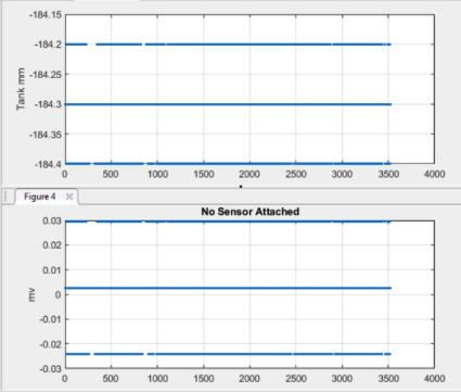
Here is an example of a data logger measuring zero volts. The bottom graph shows the measurement bouncing between bins. This is the minimum increment it can measure. The top graph converts that raw voltage measurement into mm of precipitation.

But the sensor itself also has a known repeatability: how closely it can measure the exact same height repeatedly. So the sensor number will bounce back and forth within its repeatability range, while the data logger will shift back and forth between bins.

In a worst case scenario, the bounce in the signal would be the sum of the data logger’s minimum increment and the sensor’s repeatability. However, this is rarely the case.

The precision of the data is further limited by the number of decimal places recorded. Tank depth is truncated at the tenth place, so the smallest change recorded is 0.1 mm.

How Resolution Impacts Precipitation

For tank gauges, precipitation is derived from the change in tank level. As explained above, the tank level shifts between bins of data logger resolution and with sensor repeatability. Positive shifts in tank level can be misinterpretted as additions from precipitation. When tank level consistently and quickly increases between measurements, the increases far exceed the resolution and there is little or no impact. However, when increases in tank level are small or gradual, this can lead to inflation of precipitation in a storm event, or create rain on a dry day.

As with the example of a tipping bucket above, precipitation should only accrue in whole increments. In other words, if the tank increases by one and a half increments, the half cannot be distiguished from the signal bounce and should not be counted.

Incorporating Averaging

In 2022, weather stations were reprogrammed to measure the tank level > 60 times in 3 seconds and record the average tank height. This should be enough samples so that the standard deviation equals the data logger increment, and the mean equals the bin in the center (0 volts in the graph above). However, the sensor only updates it’s signal once per second, so this only provides a very rough average of sensor repeatability. This does not change the increment (bin size) by which the data logger measures change, but it does greatly reduce the noise in the tank level by removing switching between bins.

Resolution of HJA Sensors

So the minimum increment of precipitation for tank gauges is combination of sensor repeatability and data logger resolution to the tenth place. Since the interaction is almost never linear the root sum of squares is used to combine the resolutions. This number is then reduced by the averaging instituted in 2022, but the increment is still fixed to the minimum resolution that the data logger can read.

Tipping bucket and NOAH IV sensors have a fixed increment.

Site	Logger Resolution	Sensor Precision	Root Sum of Squares Total Noise	Increment Applied	Increment w/Averaging
UPLO SA	0.0595 mm	0.1053 mm	0.12095 mm	0.1 mm	0.1 mm
CENT SA	0.1226 mm	0.1053 mm	0.16165 mm	0.2 mm	0.1 mm
VARA SA	0.1221 mm	0.1049 mm	0.16097 mm	0.2 mm	0.1 mm
CENT SH	0.158 mm	0.3166 mm	0.35388 mm	0.4 mm	0.2 mm
UPLO SH	0.158 mm	0.3166 mm	0.35388 mm	0.4 mm	0.2 mm

For more on how these numbers are derived, continue to read in the section below.

Looking at Signal Bounce

Here are some examples of the bounce we see in the signal during dry periods, but first the data needs to be loaded and the environment set up.

# must install ipympl (Ipython-matplotlib) and nodejs
from ipywidgets.embed import embed_minimal_html
from ipywidgets import Layout
import matplotlib.pyplot as plt

# Jupyter magic to make plots display interactive
%matplotlib ipympl

# expand all plots to comfortable viewing size
plt.rcParams['figure.figsize'] = [8, 5]
Layout(width='400px', height='300px')

import pandas as pd
from numpy import nan, arange, floor

import sys
sys.path.append("../../")
from post_gce_qc import qaqc, data_transfer, cross_probe_qc, main

flagged = main.main(2019, 2022, data_path='../../config_new.yaml', qa_params='../../qa_param.yaml', probes={'CEN_02'})

start, end = pd.to_datetime('9/29/19'), pd.to_datetime('10/1/19 1200')
df = flagged['CEN_02']

Loading all PPT data from ../../config_new.yaml

Load data from CEN_02

All quality checks and quality assurance rules applied to CEN_02
------------------

plt.subplot(311)
df.data.loc[start:end, 'tank_height'].plot(grid=True, label='tank height', legend=True)

plt.subplot(312)
delta_tank = df.data.loc[start:end, 'tank_height'].diff()
delta_tank.plot(grid=True, legend=True, label='change in tank height', linestyle='', marker='.')

plt.subplot(313)
df.data.loc[start:end, 'adj_precip'].plot(grid=True, label='precip', legend=True, marker='x')

<Axes: xlabel='Date'>

This is a great example from CEN shelter. The change in tank height rarely exceeds the combined increment of 0.4 mm, but had enough positive change to generate some false precip in sub-measurable increments.

Bounce During Dry Periods

Next, we will look at dry periods that were longer than an hour and what the signal bounce looked like during these dry periods. This gives a good sense of how much noise was in the signal when the tank was flat, and how much of this noise was below the minimum increment of the data. There is likely a similar amount of noise during rainy periods, which is why it is important to round precipitation to whole increments. This also excludes periods like the example above with small amounts of false precip, which likely are derived from larger signal bounce.

zeroppt = df.data['adj_precip'] == 0

# convert zero_ppt into groups and count the size of each group.
# mark the start and stop of each continuous group
ppt_turn_onoff = zeroppt.diff()
# assign a number to each continuous group
number_continuous_grps = ppt_turn_onoff.astype('boolean').cumsum()
# returns the size of each group of consecutive values
how_many_in_group = zeroppt.groupby(number_continuous_grps).transform('size')

hour_wo_ppt = (how_many_in_group > 12) & zeroppt

tank_change =  df.data['tank_height'].diff()
drains = tank_change < -5
jumps = tank_change > 5
no_rain_no_drain = tank_change[~drains & ~jumps & hour_wo_ppt]

no_rain_no_drain.describe(percentiles=[0.05, 0.1,0.2,0.25,0.5,0.75,0.8,0.9, 0.95])

count    357288.0
mean    -0.000725
std      0.185513
min     -2.299988
5%      -0.300018
10%     -0.200012
20%         -0.16
25%     -0.100006
50%           0.0
75%      0.100006
80%          0.16
90%      0.200012
95%      0.300018
max      1.799988
Name: tank_height, dtype: double[pyarrow]

plt.figure()
no_rain_no_drain.hist(bins=50)

<Axes: >

The mean is very close to 0 and the median is 0, which confirms that the tank is flat during this period. The remaining variation in tank level is bounce, with an euqual distribution of negative and positive bounce: the 90th and 80th percentiles are the absolute values of the 10th and 20th percentiles. While 0.2 may be the 90th percentile, it accounts for ~40,000 5 minute values. It is notable that the variation during these hour long dry periods is below the combined increment of 0.4. The 0.4 increment is derived from device specifications and seems to capture the full range of bounce in each direction. Manufacturers often provde worst case numbers, and in this case it seems to line up with the outer bounds of the signal bounce in the data.

Impact of Averaging

The addition of averaging in 2022 greatly reduced signal bounce. This is obvious from a simple look at the change in tank when precip equals zero, but there is also a marked change in the histogram.

flagged = main.main(2023, 2024, data_path='../../config_new.yaml', qa_params='../../qa_param.yaml', probes={'CEN_02'})

delta_tank = flagged['CEN_02'].data['tank_height'].diff()
zero_avgppt = flagged['CEN_02'].data['adj_precip'] == 0

Loading all PPT data from ../../config_new.yaml

Load data from CEN_02

All quality checks and quality assurance rules applied to CEN_02
------------------

plt.figure()
tank_change[zeroppt].plot(grid=True, legend=True, label='Change in tank height', linestyle='', marker='.')
delta_tank[zero_avgppt].plot(grid=True, legend=True, label='Averaged change in tank height', linestyle='', marker='.')

<Axes: xlabel='Date'>

Site	SD of No Rain Tank Change	Averaged SD of No Rain Tank Change
VARA SA	0.2052 mm	0.0454 mm
UPLO SA	0.0877 mm	0.0522 mm
CENT SA	0.0855 mm	0.0504 mm
CENT SH	0.1872 mm	0.0808 mm
UPLO SH	0.2087 mm	0.0622 mm

Efforsts to Reduce Signal Noise

To help reduce signal noise and combat extremes, a number of strategies have been employed.`

1. Measurement averaging: to try and record the mean that the signal bounces around, weather stations were reprogrammed to measure each sensor multiple times over a 3 second period. Each sensor remeasures every second, and the weather stations averages 60 measurements at Shelter gauges and 86 measurements at Stand Alone gauges over the 3 second period. This creates a total of 3 sensor measurements and a minnimum of 20 measurements by the weather station logger device for each sensor measurement. This should eliminate bounce from the weather station measurement device and reduce the bounce from the sensor. See this report for proof of concept of the averaging scheme.

2. Sensor grounding: Re-grounding of sensors, equalization of grounds, and re-grounding of cable drains has been done at multiple sites to drain away any electrical interference and stabilize any electrical noise.

3. Ferrite cores have been clamped around the signal cable at multiple locations to clamp any signal noise or electrical interference.

4. Resistors used in series to measure the 4-20mA sensor signal have been replaced with new, high precision, temperature stable resistors. See this report for further explanation of how the sensor is measured.

How Big an Impact Does This Have?

Rounding data to the nearest filled increment (bin) removes precipitation that resulted from signal bounce rather than a real increase in tank level. Because only full bins are counted, this effectively rounds down the data. This impacts the data in two ways: first, it reduces precipitation during storm events, and second, it reduces marginal amounts of isolated precipitation on days that would otherwise be dry.

This is best understood by looking at:

1. The daily reduction in precip

2. The water year reduction in precip

3. The number of days per water year with 0 precip

We will look at the period without measurement averaging below. All other quality controls are applied first to make sure rounding is performed on a clean dataset.

flagged = main.main(2019, 2022, data_path='../../config_new.yaml', qa_params='../../qa_param.yaml', probes={'CEN_02'})

# get the unadjusted precip
unadj = flagged['CEN_02'].data.copy(deep=True)

# apply the increment check
increment = 0.4
scrape_remainders_window = 12
flagged['CEN_02'].round_precip_to_min_increment(increment, scrape_remainders_window )

adj = flagged['CEN_02'].data

Loading all PPT data from ../../config_new.yaml

Load data from CEN_02

All quality checks and quality assurance rules applied to CEN_02
------------------

Daily Reduction in Precip

How much precip was removed from each day where it rained?

redux = unadj['adj_precip'] - adj['adj_precip']

dly_redux = redux.resample('1D').sum()

where_redux = dly_redux > 0

dly_redux[where_redux].describe(percentiles=[0.1,0.2,0.25,0.5,0.75,0.8,0.9])

count       807.0
mean     0.595218
std      0.429854
min           0.0
10%           0.1
20%           0.2
25%          0.29
50%           0.5
75%           0.8
80%         0.938
90%         1.236
max          2.26
Name: adj_precip, dtype: double[pyarrow]

plt.figure()
dly_redux[where_redux].hist(bins=30)

<Axes: >

80% of all days where precip was reduced, it was reduced by less than 1 mm, or 0.04 in of precipitation. In the worst case, the reduction was still below 0.1 in. It is also worth noting that only 807 days had any reduction out of 1,462 total days. That leaves 655 days where there was no reduction, or 45%.

Water Year Reduction in Precip

How much precip was removed from each water year.

wy = pd.DataFrame(pd.DataFrame({'unadj':unadj['adj_precip'], 'adj':adj['adj_precip']})).groupby(pd.Grouper(freq='YE-SEP'))

wy.cumsum().plot(grid=True, legend=True)

<Axes: xlabel='Date'>

wy.sum().diff(axis=1)['adj'][:-1]

2019-09-30   -130.870028
2020-09-30   -119.400546
2021-09-30   -108.560023
2022-09-30   -121.010029
Freq: YE-SEP, Name: adj, dtype: double[pyarrow]

wy.sum().pct_change(axis=1)['adj'][:-1]

/var/folders/vs/y0_kk_gj2jxcb2z5xvlgv9g80000gq/T/ipykernel_40716/4046809217.py:1: FutureWarning: Downcasting object dtype arrays on .fillna, .ffill, .bfill is deprecated and will change in a future version. Call result.infer_objects(copy=False) instead. To opt-in to the future behavior, set `pd.set_option('future.no_silent_downcasting', True)`
  wy.sum().pct_change(axis=1)['adj'][:-1]

2019-09-30   -0.067179
2020-09-30   -0.076824
2021-09-30   -0.061958
2022-09-30   -0.056892
Freq: YE-SEP, Name: adj, dtype: float64

Number of Days Per Year Without Precipitation

How much of the reduction in precipitation comes from converting days with marginal amounts of precipitation to dry days?

unadj_day = unadj['adj_precip'].resample('1D').sum()
unadj_day[unadj_day == 0].count()

650

adj_day = adj['adj_precip'].resample('1D').sum()
adj_day[adj_day == 0].count()

866

866/650

1.3323076923076924

wy_adj_dry = adj_day[adj_day == 0].groupby(pd.Grouper(freq='YE-SEP')).count()
wy_unadj_dry = unadj_day[unadj_day == 0].groupby(pd.Grouper(freq='YE-SEP')).count()

(wy_adj_dry / wy_unadj_dry)[:-1]

2019-09-30     1.30625
2020-09-30    1.385093
2021-09-30        1.32
2022-09-30    1.320261
Freq: YE-SEP, Name: adj_precip, dtype: double[pyarrow]

That is a whopping 33% increase in the number of days without rain, and up to to a 38% increase in a single water year. Compared to the 5-8% decrease in overall precipitation, that is a lot. Now let’s look at what portion of precipitation reduction comes from these dry days.

redux = unadj['adj_precip'] - adj['adj_precip']

dly_redux = redux.resample('1D').sum()

wy_redux = dly_redux[adj_day == 0].groupby(pd.Grouper(freq='YE-SEP')).sum()
wy_redux[:-1]

2019-09-30    18.26
2020-09-30    18.02
2021-09-30    15.17
2022-09-30    13.03
Freq: YE-SEP, Name: adj_precip, dtype: double[pyarrow]

(wy_redux/wy.sum().diff(axis=1)['adj'])[:-1]

2019-09-30   -0.139528
2020-09-30   -0.150921
2021-09-30   -0.139738
2022-09-30   -0.107677
Freq: YE-SEP, dtype: double[pyarrow]

Despite the large increase in the number of days without rain created by enforcing the minimum increment, these days only represent a small proportion of the overall reduction in precipitation. The majority of the reduction in total precip is from days that continue to have rain. Days with rain also have signal bounce that can lead to false precip.

Quality Checks/Rules

Since the algorithm used to derive precipitation from tank levels does not account for sensor resolution, the methods below were developed to enforce a minimum increment of precipitation accumulation on the data. Final rules are programmed in post_gce_qc.qaqc.ApplyFlags. Parameters for each rule may vary between probes and are defined in qa_params.yaml. These rules are applied to provisional data post-GCE.

The goal is to check that precipitation only accumulates by full increments. A full increment is defined as the measurable resolution of a given sensor and data logger. For NOAH IV rain gauges and tipping buckets, this is a simple check, since partial tips of a tipping bucket should not be possible in the record. However, for tank level gauges, as described above, signal noise created by bounce in measurements can make it difficult to determine whether or not the tank level has actually increased. For this reason, when the tank level increases by less than the resolution of the sensor, it is assumed to simply be signal noise.

Round Precip to Min Increment

round_precip_to_min_increment

This method rounds down so that precip is only accumulated when an increment has been filled. This avoids inflating precipitation by rounding up partial increments. Partial increments cannot be distinguished from the bounce in the signal, so they are removed.

However, since the original derivation of precipitation from tank level did not account for sensor resolution, it is possible that consecutive time steps round off precip that would have totalled an additional increment. For example:

• 13:00 0.64 rounded to 0.4

• 13:05 0.20 rounded to 0.0

In this example, 0.24 was removed followed by 0.20 for a total of 0.44 mm removed in two consecutive time steps. It makes sense, to accumulate these removed portions over a certain time period. This also creates a useful parameter; by changing the the number of time steps assessed the amount of overall precip reduction can be fine tuned. Accumulating removed portions over a larger number of time steps lowers the overall reduction in precipitation.

Rain Day Becomes Dry Day

flagged = main.main(2019, 2022, data_path='../../config_new.yaml', qa_params='../../qa_param.yaml', probes={'CEN_02', 'CEN_01'})

Loading all PPT data from ../../config_new.yaml

Load data from CEN_01

All quality checks and quality assurance rules applied to CEN_01
------------------

Load data from CEN_02

All quality checks and quality assurance rules applied to CEN_02
------------------

day = pd.to_datetime(f'10/10/18')
end = day + pd.to_timedelta('1D')

ax1, ax2 = flagged['CEN_02'].plot_flagged_day(day, 'CEN_02', paired_tank=flagged['CEN_01'].data.tank_height)
adj.loc[day:end, 'adj_precip'].plot(ax=ax1, marker='.', label='rounded precip', color='r', grid=True)
ax1.legend(loc='lower right')

<matplotlib.legend.Legend at 0x34041fac0>

day = pd.to_datetime(f'6/8/19')
end = day + pd.to_timedelta('1D')

ax1, ax2 = flagged['CEN_02'].plot_flagged_day(day, 'CEN_02', paired_tank=flagged['CEN_01'].data.tank_height)
adj.loc[day:end, 'adj_precip'].plot(ax=ax1, marker='.', label='rounded precip', color='r', grid=True)
ax1.legend(loc='lower right')

<matplotlib.legend.Legend at 0x3408ab550>

Small Rain Event Persists

day = pd.to_datetime(f'10/30/18')
end = day + pd.to_timedelta('1D')

ax1, ax2 = flagged['CEN_02'].plot_flagged_day(day, 'CEN_02', paired_tank=flagged['CEN_01'].data.tank_height)
adj.loc[day:end, 'adj_precip'].plot(ax=ax1, marker='.', label='rounded precip', color='r', grid=True)
ax1.legend(loc='lower right')

<matplotlib.legend.Legend at 0x340037a60>

day = pd.to_datetime(f'11/24/18')
end = day + pd.to_timedelta('1D')

ax1, ax2 = flagged['CEN_02'].plot_flagged_day(day, 'CEN_02', paired_tank=flagged['CEN_01'].data.tank_height)
adj.loc[day:end, 'adj_precip'].plot(ax=ax1, marker='.', label='rounded precip', color='r', grid=True)
ax1.legend(loc='lower right')

<matplotlib.legend.Legend at 0x353dd9d50>

Rounding During Rain Events

day = pd.to_datetime(f'10/27/18')
end = day + pd.to_timedelta('1D')

ax1, ax2 = flagged['CEN_02'].plot_flagged_day(day, 'CEN_02', paired_tank=flagged['CEN_01'].data.tank_height)
adj.loc[day:end, 'adj_precip'].plot(ax=ax1, marker='.', label='rounded precip', color='r', grid=True)
ax1.legend(loc='lower right')

<matplotlib.legend.Legend at 0x353df47f0>

flagged['CEN_02'].data.loc[day:end, 'adj_precip'].sum()

5.100000098347664

adj.loc[day:end, 'adj_precip'].sum()

4.800000000000001

In this case, the only reduction in precip is during the dry part of the day.

day = pd.to_datetime(f'11/1/18')
end = day + pd.to_timedelta('1D')

ax1, ax2 = flagged['CEN_02'].plot_flagged_day(day, 'CEN_02', paired_tank=flagged['CEN_01'].data.tank_height)
adj.loc[day:end, 'adj_precip'].plot(ax=ax1, marker='.', label='rounded precip', color='r', grid=True)
ax1.legend(loc='lower right')

<matplotlib.legend.Legend at 0x340b14940>

flagged['CEN_02'].data.loc[day:end, 'adj_precip'].sum()

4.600000113248825

adj.loc[day:end, 'adj_precip'].sum()

3.2

This day, the rounded off can still be easily picked out, but it is more scattered throught the day.

day = pd.to_datetime(f'11/29/18')
end = day + pd.to_timedelta('1D')

ax1, ax2 = flagged['CEN_02'].plot_flagged_day(day, 'CEN_02', paired_tank=flagged['CEN_01'].data.tank_height)
adj.loc[day:end, 'adj_precip'].plot(ax=ax1, marker='.', label='rounded precip', color='r', grid=True)
ax1.legend(loc='lower right')

<matplotlib.legend.Legend at 0x354070610>

flagged['CEN_02'].data.loc[day:end, 'adj_precip'].sum()

5.300000086426735

adj.loc[day:end, 'adj_precip'].sum()

4.800000000000001

In this case, the 0.5 mm reduction was from the dry period early in the day, while the tank was flat but bouncy.