Precipitation Resolution and Sensor Precision

The goal of this section is to determine sensor precision, and to make sure that precipitation has a resolution that is larger than precision. Put another way, this section tries to make sure that precipitation is never smaller than what we can measure.

This section draws heavily on the work of the Precipitation Sensor Replacement Plan: Coefficient Calculation and Assessment of Past and Future Sensor Accuracy.

As has been seen in many sections of this document, if the tank level is measured 10 times, the sensor returns 10 different measurements. It will bounce up and down and back again multiple times. It can be thought of as a ruler with marks; when the tank level sits between two marks, the sensor is inconsistent about whether to round the value up or down. This makes it difficult to estimate how much precipitation has been added to the tank by a simple difference in measurements. It also makes it important that the resolution (i.e. minimum incriment) of precipitation be larger than this bounce.

Sensor error can be split into both accuracy and repeatability. The accuracy of the tank level is how close the measurement is to the actual tank level. The measurement will be offset by the accuracy, but the offset is unlikely to change between any two measurements. Precipitation is the measured change in tank level, so it won’t be affected by accuracy. However, the repeatability determines how close any two measurements will be under the same conditions. This change under, say a flat tank with no new rain, will show up as bounce and is the main source of sensor error for precipitation. The repeatability is a percentage of total sensor length converted to the relative ratio of funnel to tank size. Since both ratios and sensor length differ for stand alone v.s. shelter top gauges each has a different repeatability.

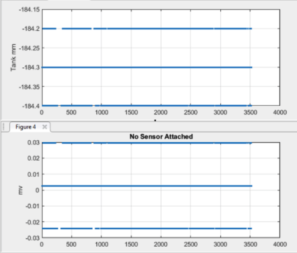
In addition to the sensor repeatability, the weather station logger has noise in measuring the sensor. This differs between the cr3000’s and cr1000’s. Here’s an example with a cr1000: with no sensor wired to the logger, this graph shows the loggers ability to measure 0 volts. In the lower graph the signal is expressed in raw millivolts; the accuracy is the small offset from 0 volts, which is nearly constant and better than listed accuracy, and the minimum precision (repeatability) is the bounce, which is just below the logger resolution of 0.033 mV. With the proper coefficient and offset applied, the logger measurement bounces +- 0.1 mm with a small difference from the sensor offset.

What’s Recorded in HJA Data

The gauges were designed to measure 0.01 in of precip, but all measurements are taken in mm with 4 significant digits. The accurate conversion into mm is an increment of 0.254, but the data loggers have a maximum precision of a 4 digit floating point (7.999, 79.99, or 799.9). Tank values are generally between 10 mm and 740 mm so measurements are mostly truncated (NOT rounded) to 0.1 mm, except when the tank is low and values are truncated to 0.01 mm. simple_pre.m then processes these tank levels into precip with the smallest increment being 0.01mm, presumably only when the tank level is low.

As shown above, a range of 0.2mm of tank change can be a flat tank and 0.1 is the smallest increment consistently included in the data. Let’s take a look and see if values below that show up much in our dataset.

# must install ipympl (Ipython-matplotlib) and nodejs
from ipywidgets.embed import embed_minimal_html
from ipywidgets import Layout
import matplotlib.pyplot as plt

# Jupyter magic to make plots display interactive
%matplotlib ipympl

# expand all plots to comfortable viewing size
plt.rcParams['figure.figsize'] = [8, 5]
Layout(width='400px', height='300px')

import pandas as pd
from numpy import nan, arange, floor
import scipy

import sys
sys.path.append("../")
from post_gce_qc import qaqc, data_transfer, cross_probe_qc, main

prov = data_transfer.LoadProvisionalData(file_n='../config_new.yaml')
prov.load_ppt_data(strtyr=2019, endyr=2024)

df = prov.pivot_on_probe(prov.df, 'UPL', '01')

non0ppt = df.TOT[df.TOT!=0]
non0ppt.describe()

count       63632.0
mean       0.596274
std        3.803037
min            0.01
25%             0.1
50%             0.2
75%             0.3
max      356.720001
Name: TOT, dtype: double[pyarrow]

So we saw in the example above that the logger by itself produces data that is +- 0.1mm, with a range of 0.2mm when the tank is flat, and 0.2 is the median increment… That doesn’t seem ideal. Notably, 0.1 is the 25th percentile and the min is as low as 0.01 mm. As stated above,that decimal place is only included when the tank level is below 79.99.

Let’s dig a little more.

tinyppt = df.TOT[(df.TOT<=0.2)&(df.TOT!=0)]
tinyppt.describe()

count     31454.0
mean     0.087867
std       0.03699
min          0.01
25%          0.08
50%           0.1
75%           0.1
max          0.19
Name: TOT, dtype: double[pyarrow]

tinyppt.groupby(pd.Grouper(freq='YE-SEP')).sum()

2019-09-30    512.609985
2020-09-30    484.080017
2021-09-30    394.200012
2022-09-30    558.049988
2023-09-30    302.350006
2024-09-30    512.489014
Freq: YE-SEP, Name: TOT, dtype: float[pyarrow]

plt.figure()
tinyppt.hist()

<Axes: >

That’s a really substantial amount of precip annually, about half of all 5 minute intervals that have precip are below the 0.2mm mark. So this small precipitation has a substantial impact. Let’s dig deeper into what the real precision of our measurments are.

What is Our Sensor Precision

Sensor precision is determined relative to sensor length, however that does not directly translate to precipitation precision since sensor depth is only a fraction of precipitation depth.

Here is the raw sensor precision, with conversion to precip explained below.

Sensor	Sensor Total Length	Sensor Measurable Length	Sites Installed	Larger of: Repeatable %	Larger of: Repeatable Max
MTS LT420	113”	105”	CENT SA, UPLO SA	0.01% (0.0105”; 0.2667mm)	0.015”; 0.381mm
MTS LT420	53”	45”	CENT SH, UPLO SH	0.01% (0.0045”; 0.1143mm)	0.015”; 0.381mm
MTS LPRefineMe	113”	105”	VARA SA	0.001% (0.00105”; 0.02667mm)	0.015”; 0.381mm

As you can see, precision is always limited by the sensor max number since it is always larger than the % of length.

Converting Tank Depth to Precip

\(PrecipDepth_{cm} = \frac{PrecipVolume_{cm^{3}}}{OrificeArea_{cm^{2}}} = \frac{TankDepth_{cm} * TankArea_{cm^{2}}}{OrificeArea_{cm^{2}}} = TankDepth_{cm} * \frac{TankArea_{cm^{2}}}{OrificeArea_{cm^{2}}}\)

TankDepth can be read directly by the sensor. TankArea is the combined area of the two tanks, minus the area of the sensor rod (the float moves up and down the rod) and the outside diameter of any copper heating pipes (the stand alone has two).

# shelter
from math import pi
def diam2A(diam):
    return pi*(diam/2)**2

# orifice area
A_or = diam2A(13.305 * 25.4)

# 2 shelter tanks equalized at base
A_tk = diam2A(6.25 * 25.4)
A_tk += diam2A(10.414 * 25.4)
# subtract sensor rod
A_tk -= diam2A(5/8. * 25.4)

A_tk / A_or

0.8310968078869966

# Stand Alone
# orifice area
A_or = diam2A(19.75 * 25.4)

# 2 shelter tanks equalized at base
A_tk = diam2A(10 * 25.4)
A_tk += diam2A(3 * 25.4)
# subtract sensor rod
A_tk -= diam2A(5/8. * 25.4)
# subtract to 2 x 1/2" heating pipes InsideDiam 0.5", OutsideDiam 5/8"
A_tk -= diam2A(5/8. * 25.4)
A_tk -= diam2A(5/8. * 25.4)

A_tk / A_or

0.27643807082198374

# VARA Stand Alone
# orifice area
A_or = diam2A(19.7917 * 25.4)

# 2 shelter tanks equalized at base
A_tk = diam2A(10 * 25.4)
A_tk += diam2A(3 * 25.4)
# subtract sensor rod
A_tk -= diam2A(5/8. * 25.4)
# subtract to 2 x 1/2" heating pipes InsideDiam 0.5", OutsideDiam 5/8"
A_tk -= diam2A(5/8. * 25.4)
A_tk -= diam2A(5/8. * 25.4)

A_tk / A_or

0.27527441901945876

Because 1 mm in tank change is only 0.27 mm of precip, the minimum repeatability of the sensor tank measurement is also reduced, increasing the precision of the measurement, with a greateer effect on the stand alone rain gauge than the shelter top gauge.

Converting Sensor Precision to Precip Precision

When the are then applied to the maximum precision of the sensor depth, the result is:

print(f'SH precision:      {0.381 * 0.8310968078869966}')
print(f'SA precision:      {0.381 * 0.27643807082198374}')
print(f'VARA SA precision: {0.381 * 0.27527441901945876}')

SH precision:      0.3166478838049457
SA precision:      0.1053229049831758
VARA SA precision: 0.10487955364641378

So the signal bounce from the sensor, translates to a lot of bounce in precip. This is especially true for the shelter top rain gauges.

What is Logger Precision

Starting in Aug-Oct of 2022, a new program was installed at station loggers to that measures the sensor at least 60 times over 3 seconds and records the average sensor measurement. Since the sensor only changes it’s amperage once per second, there is only an average of 3 sensor measurements, but 20 or more logger measurements of a sinlge sensor measurement. In testing, with no sensor attached, this created a completely flat tank measurement. As a result, any remaining signal bounce is from the sensor alone, not the logger. To account for this shift, the data must be split into pre 2022 and post 2022. The installation was close to the WY in a dry time of year, so the water year is a good dividing line. The logger precision is still important, however, to data before 2022.

Logger precision is it’s minimum microvolts (uV) of resolution in measuring the input signal. The input signal ranges from 4 - 20 milliamperes (mA) measured across a 12.4 ohm resister. The signal must also be converted from tank depth to precip. We know from the bench test above that the bounce should be 0.1 mm on a CR1000 at VARA, but let’s work it out for each configuration.

Logger	Sites Installed	Resolution
CR3000	UPLO SA	16 uV
CR1000	CENT SH; CENT SA; UPLO SH; VARA SA	33 uV

Converting Signal to mm

\(PhysicalPrecision_{mm} = SignalPrecision_{mV} * \frac{PhysicalRange_{mm}}{SignalRange_{mV}} * \frac{TankArea_{cm^{2}}}{OrificeArea_{cm^{2}}}\)

\(SignalRange = 20_{mA} - 4_{mA} = 16_{mA}\)

\(E_{mV} = R_{\ohm} * I_{mA} = 12.4_{\ohm} * 16_{mA} = 198.4_{mV}\)

\(PhysicalRange = 105 in * \frac{25.4 mm}{1 in} = 2667 mm\)

# Stand Alone mm/mv
2667/198.4

13.442540322580644

print(f"CR3000 StandAlone (UPLO) {13.442540322580644* 0.016 * 0.27643807082198374} mm")
print(f"CR1000 StandAlone (CENT) {13.442540322580644* 0.033 * 0.27643807082198374} mm")
print(f"CR1000 StandAlone (VARA) {13.442540322580644* 0.033 * 0.27527441901945876} mm")

CR3000 StandAlone (UPLO) 0.05945647861953472 mm
CR1000 StandAlone (CENT) 0.12262898715279037 mm
CR1000 StandAlone (VARA) 0.12211278675565315 mm

# Shelter mm/mv
(45*25.4)/198.4

5.761088709677419

print(f"CR1000 SH (CENT/UPLO) {5.761088709677419* 0.033 * 0.8310968078869966} mm")

CR1000 SH (CENT/UPLO) 0.15800474040670173 mm

So to summarize that:

Logger	Sensor Length	Sites Installed	Logger Resolution (mV)	Logger Resolution (mm)
CR3000	105”	UPLO SA	0.016 mV	0.05946 mm
CR1000	105”	CENT SA	0.033 mV	0.12263 mm
CR1000	105”	VARA SA	0.033 mV	0.12211 mm
CR1000	45”	CENT SH; UPLO SH	0.033 mV	0.15800 mm

This seems to match with the example from VARA above, where there was roughly 0.1 mm of bounce in each direction.

Let’s put this another way: can the logger measure the bounce in the sensor? If the sensor bounce is below the detection of the logger then all of the bounce is from the logger.

signal_range = 20 - 4
signal_range_mv = signal_range * 12.4

phys_range_mm = 105 * 25.4
mvPERmm = signal_range_mv / phys_range_mm

print(f"SA sensor bounce {0.1053229049831758 * mvPERmm} mV")

phys_range_mm = 45 * 25.4
mvPERmm = signal_range_mv / phys_range_mm
print(f"SH sensor bounce {0.3166478838049457 * mvPERmm} mV")

SA sensor bounce 0.007835044750154509 mV
SH sensor bounce 0.05496320222826004 mV

For the shelters, the sensor resolution is approaching double the logger’s resolution, so that is definitely being measured. However, at the stand alone gauges the bounce is either 1/4 or 1/2 of the logger resolution. So sometimes that won’t be measurable because the bounce will be below detection. I think this lines up with what we see at the stations: the shelters have a much noisier signal. However, the stand alones will sit steady at one level and then suddenly shift to a new level. This would make sense if they are frequently bouncing below the detectible level of the logger and then suddenly bounce above the detectible threshold.

Does Precision Match the Noise in Our Data?

Let’s grab data where there is no precip for a period of at least 1 hour.

UPLO SA

Expected Noise

The worst case scenario would be an additive noise of the sensor plus the logger, but each is independent and its shift is just as likely to be negative as a positive, so a root sum of squares may be a better estimate of the error.

print(f"Additive signal bounce {0.1053229049831758 + 0.05945647861953472}")
print(f"Root Square Sum signal bounce {(0.1053229049831758**2 + 0.05945647861953472**2)**(1/2)}")

Additive signal bounce 0.16477938360271052
Root Square Sum signal bounce 0.12094621599674074

Estimating Noise

zeroppt = df['TOT'] == 0

# `.diff()` of boolean yields True whenever consecutive rows have different boolean values
# `.cumsum()` then assigns a number at the beginning of each group.
ppt_turn_onoff = zeroppt.diff()
number_continuous_grps = ppt_turn_onoff.astype('boolean').cumsum()
# this returns the size of each group of consecutive values
how_many_in_group = zeroppt.groupby(number_continuous_grps).transform('size')
hour_wo_ppt = (how_many_in_group > 12) & zeroppt

pd.options.display.min_rows = 30
df.loc[hour_wo_ppt, 'INST']

Date
2018-10-01 00:20:00     45.029999
2018-10-01 00:25:00         44.98
2018-10-01 00:30:00     45.029999
2018-10-01 00:35:00     45.029999
2018-10-01 00:40:00     45.049999
2018-10-01 00:45:00         45.07
2018-10-01 00:50:00     44.990002
2018-10-01 00:55:00     45.049999
2018-10-01 01:00:00     45.080002
2018-10-01 01:05:00     45.080002
2018-10-01 01:10:00     45.040001
2018-10-01 01:15:00     45.040001
2018-10-01 01:20:00     45.060001
2018-10-01 01:30:00     45.009998
2018-10-01 01:35:00          45.0
                          ...
2024-09-30 22:50:00         133.5
2024-09-30 22:55:00         133.5
2024-09-30 23:00:00         133.5
2024-09-30 23:05:00         133.5
2024-09-30 23:10:00    133.600006
2024-09-30 23:15:00         133.5
2024-09-30 23:20:00         133.5
2024-09-30 23:25:00         133.5
2024-09-30 23:30:00         133.5
2024-09-30 23:35:00         133.5
2024-09-30 23:40:00         133.5
2024-09-30 23:45:00         133.5
2024-09-30 23:50:00         133.5
2024-09-30 23:55:00    133.600006
2024-10-01 00:00:00         133.5
Name: INST, Length: 508942, dtype: float[pyarrow]

df['INST'].diff()[hour_wo_ppt]

Date
2018-10-01 00:20:00       -0.07
2018-10-01 00:25:00   -0.049999
2018-10-01 00:30:00    0.049999
2018-10-01 00:35:00         0.0
2018-10-01 00:40:00        0.02
2018-10-01 00:45:00        0.02
2018-10-01 00:50:00   -0.079998
2018-10-01 00:55:00    0.059998
2018-10-01 01:00:00    0.030003
2018-10-01 01:05:00         0.0
2018-10-01 01:10:00   -0.040001
2018-10-01 01:15:00         0.0
2018-10-01 01:20:00        0.02
2018-10-01 01:30:00   -0.110001
2018-10-01 01:35:00   -0.009998
                         ...
2024-09-30 22:50:00         0.0
2024-09-30 22:55:00         0.0
2024-09-30 23:00:00         0.0
2024-09-30 23:05:00         0.0
2024-09-30 23:10:00    0.100006
2024-09-30 23:15:00   -0.100006
2024-09-30 23:20:00         0.0
2024-09-30 23:25:00         0.0
2024-09-30 23:30:00         0.0
2024-09-30 23:35:00         0.0
2024-09-30 23:40:00         0.0
2024-09-30 23:45:00         0.0
2024-09-30 23:50:00         0.0
2024-09-30 23:55:00    0.100006
2024-10-01 00:00:00   -0.100006
Name: INST, Length: 508942, dtype: float[pyarrow]

It already looks like there is a notable difference before and after the new logger averaging program started. #### Before Averaging

tank_change =  df['INST'].diff()
drains = tank_change < -5
jumps = tank_change > 5
no_rain_no_drain = tank_change[~drains & ~jumps & hour_wo_ppt]

switch = pd.to_datetime('9/30/22')
no_rain_no_drain.loc[:switch].describe()

count    337254.0
mean    -0.000386
std      0.084965
min         -4.98
25%     -0.050003
50%           0.0
75%      0.050001
max           1.5
Name: INST, dtype: double[pyarrow]

plt.figure()
no_rain_no_drain.loc[:switch].hist(bins=200)

<Axes: >

plt.figure()
df.INST[hour_wo_ppt].plot(grid=True, legend=True, label='Tank level')

<Axes: xlabel='Date'>

plt.figure()
df.INST[hour_wo_ppt].plot(grid=True, legend=True, label='Tank level')

<Axes: xlabel='Date'>

While the standard deviation is about 3/4 of the root square sum, the histogram shows a different picture, with 60,000 values of -0.1 and 60,000 of +0.1. This seems to be the real story, with a lot of bounce hidden just below the surface. This makes a strong case that increases < 0.1 should be ignored.

After Averaging

plt.figure()
no_rain_no_drain.plot(grid=True, linestyle='', marker='.')

<Axes: xlabel='Date'>

That realy paints a picture of +- 0.2mm before averaging began and +- 0.1 mm after averaging began.

(0.1**2 + (-0.1)**2)**(1./2.)

0.14142135623730953

no_rain_no_drain.loc[switch:].describe()

count    171592.0
mean     -0.00025
std      0.048204
min          -5.0
25%     -0.009998
50%           0.0
75%      0.009998
max      1.800003
Name: INST, dtype: double[pyarrow]

plt.figure()
no_rain_no_drain.loc[switch:].hist(bins=200)

<Axes: >

plt.figure()
df.INST.plot(grid=True, legend=True, label='Tank level')

<Axes: xlabel='Date'>

So before the averaging program started, the UPLO SA was averaging about 3/4 of the expected bounce in these hour long dry periods. That dropped to about half of just the sensor bounce after the averaging started. But the min and max are still pretty extreme, while the interquartile range has become very small, so the outliers are likely to be driving the standard deviation/average-bounce.

Looking at the tank, it is very noisy before the averaging was employed, with an overall bounce range of at least 0.3mm. Since the averaging has been employed, it appears to nearly always have clear daily/diurnal fluctuations. It’s possible that these were always present, but were lost in the noise of the earlier measurements. While the fluctuations are large, the noise at each point on the curve seems to be just 0.1mm. This seems to support the idea of the removal of logger bounce, but that sensor bounce remains.

CEN SH

Uplo SA has the highest precision (lowest number) of all of our stations. The shelters are much worse, let’s take a look at a shelter and see if it seems similar.

Expected Noise

print(f"Additive signal bounce {0.3166478838049457 + 0.15800474040670173 }")
print(f"Root Square Sum signal bounce {(0.3166478838049457**2 + 0.15800474040670173 **2)**(1/2)}")

Additive signal bounce 0.47465262421164744
Root Square Sum signal bounce 0.3538804604794387

Before Averaging

df = prov.pivot_on_probe(prov.df, 'CEN', '02')

zeroppt = df['TOT'] == 0

# `.diff()` of boolean yields True whenever consecutive rows have different boolean values
# `.cumsum()` then assigns a number at the beginning of each group.
ppt_turn_onoff = zeroppt.diff()
number_continuous_grps = ppt_turn_onoff.astype('boolean').cumsum()
# this returns the size of each group of consecutive values
how_many_in_group = zeroppt.groupby(number_continuous_grps).transform('size')
hour_wo_ppt = (how_many_in_group > 12) & zeroppt

tank_change =  df['INST'].diff()
drains = tank_change < -10
no_rain_no_drain = tank_change[~drains & hour_wo_ppt]

switch = pd.to_datetime('9/30/22')
no_rain_no_drain.loc[:switch].describe()

count    359840.0
mean    -0.000821
std      0.187211
min     -9.599991
25%     -0.100006
50%           0.0
75%      0.100006
max      1.799988
Name: INST, dtype: double[pyarrow]

plt.figure()
no_rain_no_drain.loc[:switch].hist(bins=150)

<Axes: >

plt.figure()
df.INST.plot(grid=True, legend=True, label='Tank Height')

<Axes: xlabel='Date'>

plt.figure()
df.INST.plot(grid=True, legend=True, label='Tank Height')

<Axes: xlabel='Date'>

Wow! That’s way worse! 30,000 to 40,000 values with +-0.2mm and a standard deviation of 0.18! So the average noise is about half of the precision measurement. Interestingly, it seems like it might also show the diurnal fluctuation.

After Averaging

no_rain_no_drain.loc[switch:].describe()

count    175459.0
mean    -0.000179
std      0.080787
min     -2.899994
25%     -0.040001
50%           0.0
75%      0.040001
max      1.950001
Name: INST, dtype: double[pyarrow]

plt.figure()
no_rain_no_drain.plot(grid=True, linestyle='', marker='.')

<Axes: xlabel='Date'>

Well that really shows a shift from +- 0.5 down to +- 0.2. These timeseries graphs, over so many years, really exagerate the number of jumps at each level, but they do show the categories very clearly. Let’s look at the histogram and see what it has to say.

plt.figure()
no_rain_no_drain.loc[switch:].hist(bins=150)

<Axes: >

plt.figure()
df.INST.plot(grid=True, legend=True, label='Tank Height')

<Axes: xlabel='Date'>

Wow! What a difference. The averaging had a big impact. When looking at the graphs, the tendency is to visually grab the range of high to low values, but jumps often seem to happen in 2 steps, rather than a single jump from the top of the range to the bottom of the range, so they are not reflected in the standard deviations. All the same, the averaging cuts all values in half.

Quick Numbers for Other Sites

df = prov.pivot_on_probe(prov.df, 'CEN', '01')

zeroppt = df['TOT'] == 0

# `.diff()` of boolean yields True whenever consecutive rows have different boolean values
# `.cumsum()` then assigns a number at the beginning of each group.
ppt_turn_onoff = zeroppt.diff()
number_continuous_grps = ppt_turn_onoff.astype('boolean').cumsum()
# this returns the size of each group of consecutive values
how_many_in_group = zeroppt.groupby(number_continuous_grps).transform('size')
hour_wo_ppt = (how_many_in_group > 12) & zeroppt

tank_change =  df['INST'].diff()
drains = tank_change < -10
no_rain_no_drain = tank_change[~drains & hour_wo_ppt]

switch = pd.to_datetime('9/30/22')
no_rain_no_drain.loc[:switch].describe()

count    356051.0
mean    -0.000327
std      0.085493
min     -7.339999
25%           0.0
50%           0.0
75%           0.0
max         2.036
Name: INST, dtype: double[pyarrow]

no_rain_no_drain.loc[switch:].describe()

count    175005.0
mean    -0.000139
std      0.050446
min     -2.610001
25%           0.0
50%           0.0
75%           0.0
max          1.58
Name: INST, dtype: double[pyarrow]

df = prov.pivot_on_probe(prov.df, 'UPL', '02')

zeroppt = df['TOT'] == 0

# `.diff()` of boolean yields True whenever consecutive rows have different boolean values
# `.cumsum()` then assigns a number at the beginning of each group.
ppt_turn_onoff = zeroppt.diff()
number_continuous_grps = ppt_turn_onoff.astype('boolean').cumsum()
# this returns the size of each group of consecutive values
how_many_in_group = zeroppt.groupby(number_continuous_grps).transform('size')
hour_wo_ppt = (how_many_in_group > 12) & zeroppt

tank_change =  df['INST'].diff()
drains = tank_change < -10
no_rain_no_drain = tank_change[~drains & hour_wo_ppt]

switch = pd.to_datetime('9/30/22')
no_rain_no_drain.loc[:switch].describe()

count    357279.0
mean    -0.001161
std      0.208689
min         -9.16
25%     -0.009998
50%           0.0
75%      0.009998
max           2.0
Name: INST, dtype: double[pyarrow]

no_rain_no_drain.loc[switch:].describe()

count    171043.0
mean    -0.000419
std      0.062214
min     -8.199982
25%     -0.010002
50%           0.0
75%      0.010002
max      0.799995
Name: INST, dtype: double[pyarrow]

df = prov.pivot_on_probe(prov.df, 'VAR', '02')

zeroppt = df['TOT'] == 0

# `.diff()` of boolean yields True whenever consecutive rows have different boolean values
# `.cumsum()` then assigns a number at the beginning of each group.
ppt_turn_onoff = zeroppt.diff()
number_continuous_grps = ppt_turn_onoff.astype('boolean').cumsum()
# this returns the size of each group of consecutive values
how_many_in_group = zeroppt.groupby(number_continuous_grps).transform('size')
hour_wo_ppt = (how_many_in_group > 12) & zeroppt

tank_change =  df['INST'].diff()
drains = tank_change < -10
no_rain_no_drain = tank_change[~drains & hour_wo_ppt]

switch = pd.to_datetime('9/30/22')
no_rain_no_drain.loc[:switch].describe()

count    333759.0
mean     -0.00707
std      0.205209
min     -9.519999
25%           0.0
50%           0.0
75%           0.0
max      7.299988
Name: INST, dtype: double[pyarrow]

no_rain_no_drain.loc[switch:].describe()

count    183549.0
mean    -0.000367
std      0.045405
min     -7.600006
25%           0.0
50%           0.0
75%           0.0
max         2.566
Name: INST, dtype: double[pyarrow]

Observed Noise Summary

Site	Logger Resolution	Sensor Precision	Root Square Total Noise	SD of No Rain Tank Change	Averaged Signal SD of No Rain Tank Change
VARA SA	0.1221 mm	0.1049 mm	0.16096 mm	0.2052 mm	0.0454 mm
UPLO SA	0.0595 mm	0.1053 mm	0.12095 mm	0.0877 mm	0.0522 mm
CENT SA	0.1226 mm	0.1053 mm	0.16165 mm	0.0855 mm	0.0504 mm
CENT SH	0.158 mm	0.3166 mm	0.35388 mm	0.1872 mm	0.0808 mm
UPLO SH	0.158 mm	0.3166 mm	0.35388 mm	0.2087 mm	0.0622 mm

This is a quick look, not comprehensive definition of sensor noise. I will refer to the standard deviation as the average noise. The sensor potential bounce can always be larger than the most frequent amuont of bounce. For example, without averaging, all sites except CENT SA have a sensor bounce that averages larger than the logger resolution. And once averaging is used at the 5 minute measurement, all sites, on average, bounce less than the logger resolution. By definition, the logger must place each measurement in bins of that increment, but the tank seems to switch, most often, by a smaller increment. This could mean that, by averaging, the sensor is firmly in one bin. And this says nothing of the measured increment that the tank increases by when it is raining.

The histograms, and even raw tank figures, are very informative here, showing a much larger bracket of values by which the signal bounces; just because the SD is smaller, doesn’t mean larger jumps don’t exist. And while, visually, the range of noise is much larger, the signal does not seem to typically jump the entire range at once, but in parts; first back to the towards a central value then diverging in the other direction. The technical definitions are theoretical maxes that may not be achieved, but the logger resolution alone is clearly not the only source of noise since the SD without averaging exceeds it. The amount of change in the SD once averaging begins really highlight how the relationship does not appear to be linear. This seems to support the use of root sum of squares rather than a linear sum of noise causing components.

Is it possible that these numbers would line up better if we used the smaller sensor precision derived from sensor length?

print(f'SH precision:      {0.1143 * 0.8310968078869966}')
print(f'SA precision:      {0.2667 * 0.27643807082198374}')
print(f'VARA SA precision: {0.02667 * 0.27527441901945876}')

SH precision:      0.09499436514148371
SA precision:      0.07372603348822306
VARA SA precision: 0.007341568755248965

print(f'SH Root Sum Square Precision:      {(0.09499436514148371**2+0.15800474040670173**2)**(1/2)}')
print(f'UPLO SA Root Sum Square Precision: {(0.07372603348822306**2+0.05945647861953472**2)**(1/2)}')
print(f'CENT SA Root Sum Square Precision: {(0.07372603348822306**2+0.12262898715279037**2)**(1/2)}')
print(f'VARA SA Root Sum Square Precision: {(0.007341568755248965**2+0.12262898715279037**2)**(1/2)}')

SH Root Sum Square Precision:      0.18436221792879023
UPLO SA Root Sum Square Precision: 0.0947132560085534
CENT SA Root Sum Square Precision: 0.14308527703445179
VARA SA Root Sum Square Precision: 0.12284855360120148

Choosing an Increment for Precip Data

The first limitation is that once the tank exceeds 79.99 mm only a single decimal place is recorded. For that reason, only 1 decimal place should be used and the increment must be at least 0.1 mm or greater.

The second limitation is the logger resolution. Changes cannot be measured below that incriment. If the noise is thought of as rounding up or down (or placing the value in one of two bins), the impact of the averaging should average which bin it is sorted into most. However, the data still must move by that incriment.

It is most difficult to know how to incorporate the sensor repeatability since the actual bounce always seems to be smaller than it. Is that a good metric of importance? However, when looking at the graphs, the full range always seems to closely match the +-, with the tank oscilating double that number. So the best strategy is probably to combine this bounce with the logger resolution.

As discussed above, the relationship between the sources of logger noise does not appear to function linearly. So the root of the sum of squares will be used to combine the sensor precisions. However, after averaging is applied, the logger resolution will be used as the minimum increment.

Rounding will reduce the amount of overall precip, so it is important not to be overly aggressive. The goal is to remove impossible, small accumulation that is solely from bounce in the tank measurement, especially on days that would otherwise have no rain, but to keep small amounts of real precip. Since jumps of the full range of 2 x +- seem rare, and don’t seem to match the data, a simple increment of combined sensor and logger precision will be used.

All values are rounded to the nearest first decimal (tenth) to match the tank floating point format.

Site	Logger Resolution	Sensor Precision	Root Square Total Noise	Increment Applied	Increment w/Averaging
UPLO SA	0.0595 mm	0.1053 mm	0.12095 mm	0.1	0.1
CENT SA	0.1226 mm	0.1053 mm	0.16165 mm	0.2	0.1
VARA SA	0.1221 mm	0.1049 mm	0.16097 mm	0.2	0.1
CENT SH	0.158 mm	0.3166 mm	0.35388 mm	0.4	0.2
UPLO SH	0.158 mm	0.3166 mm	0.35388 mm	0.4	0.2

That looks like a good start. Let’s see what it looks like when I apply that increment to the data.

Rounding to Nearest Increment

we wouldn’t want to round up, adding precipitation that didn’t fall. However, the concern with always rounding down is that totals may no longer be accurate over concsecutive periods. One can imagine a scenario where a shelter precip of 0.3 is rounded to full bins of 0.2mm, and removes 0.1 mm in two consecutive measurements. While the 5 minute measurements of 0.3 are below precision to measure, the 10 minute total of 0.6 mm is not below detection. So, when rounding down the 0.3 accumulation, the amount removed must be tracked and accumulated over some time frame.

So the values rounding off must be tracked and accumulated over some period.

First, the rounding must be adjusted from nearest to rounding down.

Check Rounding: Floating Point Errors

%reload_ext autoreload
%aimport post_gce_qc.qaqc

from importlib import reload

reload(post_gce_qc.qaqc)

params = qaqc._load_yaml('../qa_param.yaml')['UPL_02']
qc = qaqc.QaRules(df, params)

from numpy import floor
real_ppt = qc.round_to_precision(df.TOT, 0.4, round_fnc=floor)

remainder = df.TOT - real_ppt

remainder[remainder!=0].describe()

count     46443.0
mean     0.173104
std      0.102457
min           0.0
25%           0.1
50%           0.2
75%          0.25
max           0.4
Name: TOT, dtype: double[pyarrow]

any(remainder>=0.4)

False

any(remainder>=0.39999)

True

??? what?? Nothing should be rounded down from 0.4. Let’s dig into the issue.

df[remainder>=0.3999999]

	INST	INST_Flag	TOT	TOT_Flag	ACC	ACC_Flag
Date
2020-03-26 12:30:00	91.300003	Q	2.8	<NA>	1452.5	<NA>
2020-09-05 08:35:00	30.219999	Q	2.8	<NA>	7836.400391	<NA>
2020-10-03 18:55:00	707.299988	Q	2.8	<NA>	2987.5	<NA>
2020-10-03 19:55:00	709.900024	Q	2.8	<NA>	3006.500244	<NA>
2020-10-03 21:10:00	701.900024	Q	3.6	<NA>	3032.400146	<NA>
2020-10-03 22:30:00	708.200012	Q	2.8	<NA>	3078.500244	<NA>
2020-10-04 01:45:00	706.5	Q	7.6	<NA>	3137.800049	<NA>
2020-10-04 07:30:00	703.900024	Q	3.6	<NA>	3273.800049	<NA>
2020-10-04 09:55:00	700.599976	Q	2.8	<NA>	3338.899902	<NA>
2020-10-04 18:10:00	699.400024	Q	2.8	<NA>	3767.0	<NA>
2020-10-04 23:50:00	696.799988	Q	3.6	<NA>	3863.599854	<NA>
2020-10-05 04:45:00	697.099976	Q	2.8	<NA>	3883.899902	<NA>
2020-10-05 05:55:00	691.5	Q	5.6	<NA>	3892.099854	<NA>
2020-10-05 10:15:00	699.599976	Q	2.8	<NA>	3942.099854	<NA>
2020-10-05 14:25:00	696.299988	Q	2.8	<NA>	4058.299805	<NA>
...	...	...	...	...	...	...
2021-07-28 12:20:00	517.200012	Q	3.6	<NA>	87788.234375	<NA>
2021-07-29 18:45:00	452.899994	Q	5.6	J	88461.335938	J
2021-07-29 19:50:00	456.5	Q	3.6	<NA>	88577.4375	<NA>
2021-07-30 09:35:00	490.200012	Q	2.8	<NA>	88718.835938	<NA>
2021-07-31 07:15:00	480.200012	Q	2.8	<NA>	88818.9375	<NA>
2021-07-31 16:10:00	485.5	Q	3.6	<NA>	88870.632812	<NA>
2021-08-01 20:05:00	461.700012	Q	3.6	<NA>	89862.632812	<NA>
2021-08-01 20:25:00	465.5	Q	2.8	<NA>	89871.132812	<NA>
2021-08-01 22:10:00	473.100006	Q	2.8	<NA>	89906.4375	<NA>
2021-08-02 00:45:00	477.200012	Q	5.6	J	89970.4375	J
2021-08-02 02:35:00	478.700012	Q	5.6	J	90017.234375	J
2021-08-02 04:45:00	475.200012	Q	3.6	<NA>	90063.539062	<NA>
2023-10-12 09:35:00	204.399994	Q	2.8	<NA>	107.800003	<NA>
2023-11-15 13:10:00	231.0	Q	5.6	J	369.799988	J
2024-01-10 09:40:00	190.699997	Q	2.8	<NA>	1085.115967	<NA>

353 rows × 6 columns

real_ppt[remainder>=0.39999]

Date
2020-03-26 12:30:00      2.4
2020-06-14 07:05:00     26.4
2020-09-05 08:35:00      2.4
2020-10-02 11:55:00     16.0
2020-10-02 12:45:00     34.4
2020-10-02 13:45:00     22.0
2020-10-02 17:35:00      6.8
2020-10-02 21:05:00     16.0
2020-10-02 22:35:00     30.4
2020-10-03 12:25:00     10.0
2020-10-03 16:20:00     20.4
2020-10-03 18:55:00      2.4
2020-10-03 19:55:00      2.4
2020-10-03 21:10:00      3.2
2020-10-03 21:25:00     10.0
                       ...
2021-07-31 16:10:00      3.2
2021-08-01 12:05:00     10.0
2021-08-01 13:55:00      6.8
2021-08-01 14:05:00     52.4
2021-08-01 20:05:00      3.2
2021-08-01 20:25:00      2.4
2021-08-01 22:10:00      2.4
2021-08-02 00:45:00      5.2
2021-08-02 01:35:00      8.0
2021-08-02 02:35:00      5.2
2021-08-02 04:45:00      3.2
2021-12-29 15:25:00    196.0
2023-10-12 09:35:00      2.4
2023-11-15 13:10:00      5.2
2024-01-10 09:40:00      2.4
Name: TOT, Length: 705, dtype: float64

3.6/0.4

9.0

floor(3.6/0.4)

9.0

9*0.4

3.6

0.4*floor(3.6/0.4)

3.6

sr = pd.Series([3.6, 3.2, 2.8, 2.4, 2.0, 0.4, 0.8])
sr/0.4

0    9.0
1    8.0
2    7.0
3    6.0
4    5.0
5    1.0
6    2.0
dtype: float64

floor(sr/0.4)

0    9.0
1    8.0
2    6.0
3    5.0
4    5.0
5    1.0
6    2.0
dtype: float64

2.8/0.4

6.999999999999999

(sr).floordiv(0.4)

0    8.0
1    8.0
2    6.0
3    5.0
4    4.0
5    1.0
6    2.0
dtype: float64

This only appears to happen once, but this lack of precision in the 64 bit float does cause a problem. Let’s see about pre-rounding.

round(sr/0.4, ndigits=5)

0    9.0
1    8.0
2    7.0
3    6.0
4    5.0
5    1.0
6    2.0
dtype: float64

floor(round(sr/0.4, ndigits=5))

0    9.0
1    8.0
2    7.0
3    6.0
4    5.0
5    1.0
6    2.0
dtype: float64

reload(post_gce_qc.qaqc)
real_ppt = qc.round_to_precision(df.TOT, 0.4, round_fnc=floor)

remainder = df.TOT - real_ppt
remainder[remainder!=0].describe()

count     46443.0
mean     0.173104
std      0.102457
min           0.0
25%           0.1
50%           0.2
75%          0.25
max           0.4
Name: TOT, dtype: double[pyarrow]

df.loc[remainder>=0.3999, 'TOT'].values

<ArrowExtensionArray>
[ 2.799999952316284, 26.799999237060547,  2.799999952316284,
 16.399999618530273,  34.79999923706055, 22.399999618530273,
  7.199999809265137, 16.399999618530273, 30.799999237060547,
 10.399999618530273,
 ...
  2.799999952316284,  5.599999904632568,  8.399999618530273,
  5.599999904632568, 3.5999999046325684, 278.79998779296875,
 196.39999389648438,  2.799999952316284,  5.599999904632568,
  2.799999952316284]
Length: 707, dtype: float[pyarrow]

Ahhh. OK, so the raw data needs to be rounded back to 4 decimal places for this to work.

reload(post_gce_qc.qaqc)
real_ppt = qc.round_to_precision(df.TOT, 0.4, round_fnc=floor)

remainder = df.TOT - real_ppt
remainder[remainder!=0].describe()

count     46443.0
mean     0.173104
std      0.102457
min           0.0
25%           0.1
50%           0.2
75%          0.25
max           0.4
Name: TOT, dtype: double[pyarrow]

OK, we still have a problem number in there.

df.loc[remainder>=0.3999, 'TOT'].values

<ArrowExtensionArray>
[ 2.799999952316284, 26.799999237060547,  2.799999952316284,
 16.399999618530273,  34.79999923706055, 22.399999618530273,
  7.199999809265137, 16.399999618530273, 30.799999237060547,
 10.399999618530273,
 ...
  2.799999952316284,  5.599999904632568,  8.399999618530273,
  5.599999904632568, 3.5999999046325684, 278.79998779296875,
 196.39999389648438,  2.799999952316284,  5.599999904632568,
  2.799999952316284]
Length: 707, dtype: float[pyarrow]

round(df.loc[remainder>=0.3999, 'TOT'], 4).values

<ArrowExtensionArray>
[ 2.799999952316284, 26.799999237060547,  2.799999952316284,
 16.399999618530273,  34.79999923706055, 22.399999618530273,
  7.199999809265137, 16.399999618530273, 30.799999237060547,
 10.399999618530273,
 ...
  2.799999952316284,  5.599999904632568,  8.399999618530273,
  5.599999904632568, 3.5999999046325684, 278.79998779296875,
 196.39999389648438,  2.799999952316284,  5.599999904632568,
  2.799999952316284]
Length: 707, dtype: float[pyarrow]

round(df.loc[remainder>=0.3999, 'TOT'],4)*10000

Date
2020-03-26 12:30:00      28000.0
2020-06-14 07:05:00     268000.0
2020-09-05 08:35:00      28000.0
2020-10-02 11:55:00     164000.0
2020-10-02 12:45:00     348000.0
2020-10-02 13:45:00     224000.0
2020-10-02 17:35:00      72000.0
2020-10-02 21:05:00     164000.0
2020-10-02 22:35:00     308000.0
2020-10-03 12:25:00     104000.0
2020-10-03 16:20:00     208000.0
2020-10-03 18:55:00      28000.0
2020-10-03 19:55:00      28000.0
2020-10-03 21:10:00      36000.0
2020-10-03 21:25:00     104000.0
                         ...
2021-08-01 12:05:00     104000.0
2021-08-01 13:55:00      72000.0
2021-08-01 14:05:00     528000.0
2021-08-01 20:05:00      36000.0
2021-08-01 20:25:00      28000.0
2021-08-01 22:10:00      28000.0
2021-08-02 00:45:00      56000.0
2021-08-02 01:35:00      84000.0
2021-08-02 02:35:00      56000.0
2021-08-02 04:45:00      36000.0
2021-08-02 08:25:00    2788000.0
2021-12-29 15:25:00    1964000.0
2023-10-12 09:35:00      28000.0
2023-11-15 13:10:00      56000.0
2024-01-10 09:40:00      28000.0
Name: TOT, Length: 707, dtype: float[pyarrow]

(round(df.loc[remainder>=0.3999, 'TOT'],4)*10000).values

<ArrowExtensionArray>
[  28000.0,  268000.0,   28000.0,  164000.0,  348000.0,  224000.0,   72000.0,
  164000.0,  308000.0,  104000.0,
 ...
   28000.0,   56000.0,   84000.0,   56000.0,   36000.0, 2788000.0, 1964000.0,
   28000.0,   56000.0,   28000.0]
Length: 707, dtype: float[pyarrow]

(round(df.loc[remainder>=0.3999, 'TOT'],4)*10000 / (0.4 * 10000)).values

<ArrowExtensionArray>
[  7.0,  67.0,   7.0,  41.0,  87.0,  56.0,  18.0,  41.0,  77.0,  26.0,
 ...
   7.0,  14.0,  21.0,  14.0,   9.0, 697.0, 491.0,   7.0,  14.0,   7.0]
Length: 707, dtype: double[pyarrow]

reload(post_gce_qc.qaqc)
real_ppt = qc.round_to_precision(df.TOT, 0.4, round_fnc=floor)

remainder = df.TOT - real_ppt
remainder[remainder!=0].describe()

count     46443.0
mean     0.173104
std      0.102457
min           0.0
25%           0.1
50%           0.2
75%          0.25
max           0.4
Name: TOT, dtype: double[pyarrow]

df.loc[remainder>=0.3999, 'TOT']

Date
2020-03-26 12:30:00           2.8
2020-06-14 07:05:00     26.799999
2020-09-05 08:35:00           2.8
2020-10-02 11:55:00          16.4
2020-10-02 12:45:00     34.799999
2020-10-02 13:45:00          22.4
2020-10-02 17:35:00           7.2
2020-10-02 21:05:00          16.4
2020-10-02 22:35:00     30.799999
2020-10-03 12:25:00          10.4
2020-10-03 16:20:00     20.799999
2020-10-03 18:55:00           2.8
2020-10-03 19:55:00           2.8
2020-10-03 21:10:00           3.6
2020-10-03 21:25:00          10.4
                          ...
2021-08-01 12:05:00          10.4
2021-08-01 13:55:00           7.2
2021-08-01 14:05:00     52.799999
2021-08-01 20:05:00           3.6
2021-08-01 20:25:00           2.8
2021-08-01 22:10:00           2.8
2021-08-02 00:45:00           5.6
2021-08-02 01:35:00           8.4
2021-08-02 02:35:00           5.6
2021-08-02 04:45:00           3.6
2021-08-02 08:25:00    278.799988
2021-12-29 15:25:00    196.399994
2023-10-12 09:35:00           2.8
2023-11-15 13:10:00           5.6
2024-01-10 09:40:00           2.8
Name: TOT, Length: 707, dtype: float[pyarrow]

df_int = round(df['TOT'], ndigits=4) * 10**4
prec_int = 0.4 * 10**4
nsteps = round(df_int / prec_int, ndigits=4)
# round in the direction desired (round, ceil, floor)
n_steps = floor(nsteps)

rounded =  n_steps * 0.4
remainder = df.TOT - rounded
remainder[remainder!=0].describe()

count     46443.0
mean     0.167015
std      0.100662
min     -0.000012
25%           0.1
50%           0.2
75%          0.25
max         0.398
Name: TOT, dtype: double[pyarrow]

df.loc[remainder>=0.399, 'TOT']

Series([], Name: TOT, dtype: float[pyarrow])

Well, I copy pasted that directly from the function in qaqc.QaRules, and it doesn’t have anywhere that it rounded down by 0.4, which wouldn’t make any sense. But it does have still have that one 3.6 precip at the same timestamp which isn’t being rounded to 9 levels of precision.

This is a pretty small problems list, so, for the time being, I’m going to let it be and move on.

Accumulating What Rounded Off

The NOAH IV program, developed by ETI, waits for 15 minutes, then sees if the tank is more than 0.005 in above the reference level, then rounds up or down to 0.01 in. The notes say it waits for 30 min, but that does not match the code.

I will start by using a 15 min interval for allowing accumulation of rounded off precip. But we don’t want to count any precip more than once.

The simple rounding down (to full buckets) took a lot of precip off…

remainder.groupby(pd.Grouper(freq='YE-SEP')).sum()

2019-09-30    1725.220023
2020-09-30    1108.239956
2021-09-30     2557.33995
2022-09-30     342.603998
2023-09-30     745.257014
2024-09-30    1278.028001
2025-09-30            0.0
Freq: YE-SEP, Name: TOT, dtype: double[pyarrow]

acc_remainders = remainder.rolling('15min').sum()

acc_remainders[acc_remainders>0].describe()

count    8.792800e+04
mean     2.646491e-01
std      1.843391e-01
min      5.960464e-09
25%      1.000000e-01
50%      2.400000e-01
75%      3.500000e-01
max      1.110000e+00
Name: TOT, dtype: float64

plt.figure()
acc_remainders[acc_remainders>0].hist()

<Axes: >

df.TOT

Date
2018-10-01 00:05:00    0.0
2018-10-01 00:10:00    0.0
2018-10-01 00:15:00    0.0
2018-10-01 00:20:00    0.0
2018-10-01 00:25:00    0.0
2018-10-01 00:30:00    0.0
2018-10-01 00:35:00    0.0
2018-10-01 00:40:00    0.0
2018-10-01 00:45:00    0.0
2018-10-01 00:50:00    0.0
2018-10-01 00:55:00    0.0
2018-10-01 01:00:00    0.0
2018-10-01 01:05:00    0.0
2018-10-01 01:10:00    0.0
2018-10-01 01:15:00    0.0
                      ...
2024-09-30 22:50:00    0.0
2024-09-30 22:55:00    0.0
2024-09-30 23:00:00    0.0
2024-09-30 23:05:00    0.0
2024-09-30 23:10:00    0.0
2024-09-30 23:15:00    0.0
2024-09-30 23:20:00    0.0
2024-09-30 23:25:00    0.0
2024-09-30 23:30:00    0.0
2024-09-30 23:35:00    0.0
2024-09-30 23:40:00    0.0
2024-09-30 23:45:00    0.0
2024-09-30 23:50:00    0.0
2024-09-30 23:55:00    0.0
2024-10-01 00:00:00    0.0
Name: TOT, Length: 631296, dtype: float[pyarrow]

acc_remainders

Date
2018-10-01 00:05:00    0.0
2018-10-01 00:10:00    0.0
2018-10-01 00:15:00    0.0
2018-10-01 00:20:00    0.0
2018-10-01 00:25:00    0.0
2018-10-01 00:30:00    0.0
2018-10-01 00:35:00    0.0
2018-10-01 00:40:00    0.0
2018-10-01 00:45:00    0.0
2018-10-01 00:50:00    0.0
2018-10-01 00:55:00    0.0
2018-10-01 01:00:00    0.0
2018-10-01 01:05:00    0.0
2018-10-01 01:10:00    0.0
2018-10-01 01:15:00    0.0
                      ...
2024-09-30 22:50:00    0.0
2024-09-30 22:55:00    0.0
2024-09-30 23:00:00    0.0
2024-09-30 23:05:00    0.0
2024-09-30 23:10:00    0.0
2024-09-30 23:15:00    0.0
2024-09-30 23:20:00    0.0
2024-09-30 23:25:00    0.0
2024-09-30 23:30:00    0.0
2024-09-30 23:35:00    0.0
2024-09-30 23:40:00    0.0
2024-09-30 23:45:00    0.0
2024-09-30 23:50:00    0.0
2024-09-30 23:55:00    0.0
2024-10-01 00:00:00    0.0
Name: TOT, Length: 631296, dtype: float64

So the goal is to add 0.49 back, but only at 0015, and not at 0020.

add_ppt = acc_remainders >= 0.4

after_add = pd.Series(index=add_ppt.index, data=False)
for lookahead in range(1,3+1):
    after_add |= add_ppt.shift(lookahead)

after_add

Date
2018-10-01 00:05:00    False
2018-10-01 00:10:00    False
2018-10-01 00:15:00    False
2018-10-01 00:20:00    False
2018-10-01 00:25:00    False
2018-10-01 00:30:00    False
2018-10-01 00:35:00    False
2018-10-01 00:40:00    False
2018-10-01 00:45:00    False
2018-10-01 00:50:00    False
2018-10-01 00:55:00    False
2018-10-01 01:00:00    False
2018-10-01 01:05:00    False
2018-10-01 01:10:00    False
2018-10-01 01:15:00    False
                       ...
2024-09-30 22:50:00    False
2024-09-30 22:55:00    False
2024-09-30 23:00:00    False
2024-09-30 23:05:00    False
2024-09-30 23:10:00    False
2024-09-30 23:15:00    False
2024-09-30 23:20:00    False
2024-09-30 23:25:00    False
2024-09-30 23:30:00    False
2024-09-30 23:35:00    False
2024-09-30 23:40:00    False
2024-09-30 23:45:00    False
2024-09-30 23:50:00    False
2024-09-30 23:55:00    False
2024-10-01 00:00:00    False
Length: 631296, dtype: bool

add_ppt & ~after_add

Date
2018-10-01 00:05:00    False
2018-10-01 00:10:00    False
2018-10-01 00:15:00    False
2018-10-01 00:20:00    False
2018-10-01 00:25:00    False
2018-10-01 00:30:00    False
2018-10-01 00:35:00    False
2018-10-01 00:40:00    False
2018-10-01 00:45:00    False
2018-10-01 00:50:00    False
2018-10-01 00:55:00    False
2018-10-01 01:00:00    False
2018-10-01 01:05:00    False
2018-10-01 01:10:00    False
2018-10-01 01:15:00    False
                       ...
2024-09-30 22:50:00    False
2024-09-30 22:55:00    False
2024-09-30 23:00:00    False
2024-09-30 23:05:00    False
2024-09-30 23:10:00    False
2024-09-30 23:15:00    False
2024-09-30 23:20:00    False
2024-09-30 23:25:00    False
2024-09-30 23:30:00    False
2024-09-30 23:35:00    False
2024-09-30 23:40:00    False
2024-09-30 23:45:00    False
2024-09-30 23:50:00    False
2024-09-30 23:55:00    False
2024-10-01 00:00:00    False
Length: 631296, dtype: bool

That worked! Let’s find another example.

strt, end = pd.to_datetime('10/5/18 1905'), pd.to_datetime('10/5/18 2110')
df.loc[strt:end, ['INST', 'TOT']]

	INST	TOT
Date
2018-10-05 19:05:00	45.599998	0.25
2018-10-05 19:10:00	45.59	0.0
2018-10-05 19:15:00	45.849998	0.25
2018-10-05 19:20:00	45.84	0.0
2018-10-05 19:25:00	46.099998	0.25
2018-10-05 19:30:00	46.360001	0.26
2018-10-05 19:35:00	46.34	0.0
2018-10-05 19:40:00	46.59	0.23
2018-10-05 19:45:00	46.59	0.0
2018-10-05 19:50:00	46.580002	0.0
2018-10-05 19:55:00	47.07	0.48
2018-10-05 20:00:00	47.330002	0.26
2018-10-05 20:05:00	47.580002	0.25
2018-10-05 20:10:00	47.57	0.0
2018-10-05 20:15:00	47.830002	0.25
2018-10-05 20:20:00	47.830002	0.0
2018-10-05 20:25:00	48.07	0.24
2018-10-05 20:30:00	48.32	0.25
2018-10-05 20:35:00	48.580002	0.26
2018-10-05 20:40:00	48.830002	0.25
2018-10-05 20:45:00	49.07	0.24
2018-10-05 20:50:00	49.32	0.25
2018-10-05 20:55:00	49.580002	0.26
2018-10-05 21:00:00	49.830002	0.25
2018-10-05 21:05:00	50.209999	0.38
2018-10-05 21:10:00	50.580002	0.37

remainder[strt:end]

Date
2018-10-05 19:05:00    0.25
2018-10-05 19:10:00     0.0
2018-10-05 19:15:00    0.25
2018-10-05 19:20:00     0.0
2018-10-05 19:25:00    0.25
2018-10-05 19:30:00    0.26
2018-10-05 19:35:00     0.0
2018-10-05 19:40:00    0.23
2018-10-05 19:45:00     0.0
2018-10-05 19:50:00     0.0
2018-10-05 19:55:00    0.08
2018-10-05 20:00:00    0.26
2018-10-05 20:05:00    0.25
2018-10-05 20:10:00     0.0
2018-10-05 20:15:00    0.25
2018-10-05 20:20:00     0.0
2018-10-05 20:25:00    0.24
2018-10-05 20:30:00    0.25
2018-10-05 20:35:00    0.26
2018-10-05 20:40:00    0.25
2018-10-05 20:45:00    0.24
2018-10-05 20:50:00    0.25
2018-10-05 20:55:00    0.26
2018-10-05 21:00:00    0.25
2018-10-05 21:05:00    0.38
2018-10-05 21:10:00    0.37
Name: TOT, dtype: double[pyarrow]

acc_remainders[strt:end]

Date
2018-10-05 19:05:00    0.50
2018-10-05 19:10:00    0.25
2018-10-05 19:15:00    0.50
2018-10-05 19:20:00    0.25
2018-10-05 19:25:00    0.50
2018-10-05 19:30:00    0.51
2018-10-05 19:35:00    0.51
2018-10-05 19:40:00    0.49
2018-10-05 19:45:00    0.23
2018-10-05 19:50:00    0.23
2018-10-05 19:55:00    0.08
2018-10-05 20:00:00    0.34
2018-10-05 20:05:00    0.59
2018-10-05 20:10:00    0.51
2018-10-05 20:15:00    0.50
2018-10-05 20:20:00    0.25
2018-10-05 20:25:00    0.49
2018-10-05 20:30:00    0.49
2018-10-05 20:35:00    0.75
2018-10-05 20:40:00    0.76
2018-10-05 20:45:00    0.75
2018-10-05 20:50:00    0.74
2018-10-05 20:55:00    0.75
2018-10-05 21:00:00    0.76
2018-10-05 21:05:00    0.89
2018-10-05 21:10:00    1.00
Name: TOT, dtype: float64

add_it = add_ppt & ~after_add
add_it[strt:end]

Date
2018-10-05 19:05:00     True
2018-10-05 19:10:00    False
2018-10-05 19:15:00    False
2018-10-05 19:20:00    False
2018-10-05 19:25:00    False
2018-10-05 19:30:00    False
2018-10-05 19:35:00    False
2018-10-05 19:40:00    False
2018-10-05 19:45:00    False
2018-10-05 19:50:00    False
2018-10-05 19:55:00    False
2018-10-05 20:00:00    False
2018-10-05 20:05:00     True
2018-10-05 20:10:00    False
2018-10-05 20:15:00    False
2018-10-05 20:20:00    False
2018-10-05 20:25:00    False
2018-10-05 20:30:00    False
2018-10-05 20:35:00    False
2018-10-05 20:40:00    False
2018-10-05 20:45:00    False
2018-10-05 20:50:00    False
2018-10-05 20:55:00    False
2018-10-05 21:00:00    False
2018-10-05 21:05:00    False
2018-10-05 21:10:00    False
dtype: bool

That’s missing a few at the end.

add_ppt[strt:end]

Date
2018-10-05 19:05:00     True
2018-10-05 19:10:00    False
2018-10-05 19:15:00     True
2018-10-05 19:20:00    False
2018-10-05 19:25:00     True
2018-10-05 19:30:00     True
2018-10-05 19:35:00     True
2018-10-05 19:40:00     True
2018-10-05 19:45:00    False
2018-10-05 19:50:00    False
2018-10-05 19:55:00    False
2018-10-05 20:00:00    False
2018-10-05 20:05:00     True
2018-10-05 20:10:00     True
2018-10-05 20:15:00     True
2018-10-05 20:20:00    False
2018-10-05 20:25:00     True
2018-10-05 20:30:00     True
2018-10-05 20:35:00     True
2018-10-05 20:40:00     True
2018-10-05 20:45:00     True
2018-10-05 20:50:00     True
2018-10-05 20:55:00     True
2018-10-05 21:00:00     True
2018-10-05 21:05:00     True
2018-10-05 21:10:00     True
Name: TOT, dtype: bool

OK, that logic doesn’t work, because everything is True in a row. I might need to make my own rolling window… #### Custom Rolling Window There doesn’t appear to be a vectorized approach. This attempts to make an efficient rolling window by using numpy. It should be possible to use a JIT compiler to speed up the window.

import numpy as np

def rolling_sum_first_use(arr, window, threshold):
    nrow = len(arr)
    window_sum = np.zeros(nrow, dtype=np.float_)
    used = np.zeros(nrow, dtype=np.bool_)   # True = exclude from future sums
    remainder = np.zeros(nrow, dtype=np.float_)

    # for each row
    for row in range(nrow):
        # Compute sum of last `window` values, excluding masked ones
        start = max(0, row - window + 1)
        end = row + 1
        tot = 0.0
        for i in range(start, end):
            if not used[i]:
                tot += arr[i]
                tot += remainder[i]
            #remainder[i] -= remainder[i]

        if tot >= threshold:
            used[start:end] = True
            prec_tot = qaqc.QaRules.round_to_precision(tot, threshold, floor)

            window_sum[row] = prec_tot
            remainder[row + 1] = tot - prec_tot

    return window_sum

acc_remainders = rolling_sum_first_use(remainder.to_numpy(), 3, 0.4)
pd.Series(data=acc_remainders, index=remainder.index)[strt:end]

Date
2018-10-05 19:05:00    0.4
2018-10-05 19:10:00    0.0
2018-10-05 19:15:00    0.0
2018-10-05 19:20:00    0.0
2018-10-05 19:25:00    0.4
2018-10-05 19:30:00    0.0
2018-10-05 19:35:00    0.0
2018-10-05 19:40:00    0.4
2018-10-05 19:45:00    0.0
2018-10-05 19:50:00    0.0
2018-10-05 19:55:00    0.0
2018-10-05 20:00:00    0.0
2018-10-05 20:05:00    0.4
2018-10-05 20:10:00    0.0
2018-10-05 20:15:00    0.4
2018-10-05 20:20:00    0.0
2018-10-05 20:25:00    0.0
2018-10-05 20:30:00    0.4
2018-10-05 20:35:00    0.0
2018-10-05 20:40:00    0.4
2018-10-05 20:45:00    0.4
2018-10-05 20:50:00    0.0
2018-10-05 20:55:00    0.4
2018-10-05 21:00:00    0.4
2018-10-05 21:05:00    0.4
2018-10-05 21:10:00    0.0
dtype: float64

I think that’s working now. And it takes any rounded off portion of the accumulated remainders and allows it to be added back again in the next window. Let’s see if we can compile it with numbas to add a little speed. #### Numba Compile

import numba

@numba.jit
def rolling_sum_first_use_numba(arr, window, threshold):
    nrow = len(arr)
    window_sum = np.zeros(nrow, dtype=np.float_)
    used = np.zeros(nrow, dtype=np.bool_)   # True = exclude from future sums
    remainder = np.zeros(nrow, dtype=np.float_)

    # for each row
    for row in range(nrow):
        # Compute sum of last `window` values, excluding masked ones
        start = max(0, row - window + 1)
        end = row + 1
        tot = 0.0
        for i in range(start, end):
            if not used[i]:
                tot += arr[i]
                tot += remainder[i]
            #remainder[i] -= remainder[i]

        if tot >= threshold:
            used[start:end] = True
            with numba.objmode(prec_tot='float64'):
                prec_tot = qaqc.QaRules.round_to_precision(tot, threshold, floor)

            window_sum[row] = prec_tot
            remainder[row + 1] = tot - prec_tot

    return window_sum

%timeit acc_remainders = rolling_sum_first_use(remainder.to_numpy(), 3, 0.4)

323 ms ± 5.57 ms per loop (mean ± std. dev. of 7 runs, 1 loop each)

First qaqc.QaRules.round_to_precision needs to be altered to be jit compiled. Let’s also time it alone.

reload(qaqc)
%aimport post_gce_qc.qaqc

import post_gce_qc.qaqc
qaqc.ApplyFlags.rolling_accumulate_increment.recompile()

qaqc.QaRules.round_to_precision(3.5648, 0.254, floor)

3.556

%timeit qaqc.QaRules.round_to_precision(remainder, 0.4, floor)

4.06 ms ± 152 μs per loop (mean ± std. dev. of 7 runs, 100 loops each)

%%timeit
acc_remainders = rolling_sum_first_use_numba(remainder.to_numpy(), 3, 0.4)

5.15 ms ± 55 μs per loop (mean ± std. dev. of 7 runs, 100 loops each)

%%timeit
acc_remainders = rolling_sum_first_use_numba(remainder.to_numpy(), 3, 0.4)

5.27 ms ± 194 μs per loop (mean ± std. dev. of 7 runs, 100 loops each)

60 times faster with numba seems worth it. Adding 1/3 of a second to processing for each site was pretty excessive. That took a little bit of work to get it to use the round function though. Basically, the round function must first be JustInTime (jit) compiled, and it didn’t wan’t to compile with a method object as an input. The key was to force it compile as a python object instead of as a raw vectorized function. Then it needs to be sepcified as an object when it is called from the other function.

How Big is the Reduction in Precip

CENT SH

final_remainder = df.TOT - (rounded + acc_remainders)

final_remainder.describe()

count    631296.0
mean     0.005512
std       0.04643
min          -0.4
25%           0.0
50%           0.0
75%           0.0
max         0.398
Name: TOT, dtype: double[pyarrow]

final_remainder[final_remainder>0].describe()

count     35047.0
mean     0.146535
std      0.095829
min           0.0
25%           0.1
50%          0.11
75%           0.2
max         0.398
Name: TOT, dtype: double[pyarrow]

final_remainder.groupby(pd.Grouper(freq='YE-SEP')).sum()

2019-09-30    622.020023
2020-09-30    488.639956
2021-09-30    1507.33995
2022-09-30    125.403998
2023-09-30    283.257014
2024-09-30    452.828001
2025-09-30           0.0
Freq: YE-SEP, Name: TOT, dtype: double[pyarrow]

(rounded + acc_remainders).groupby(pd.Grouper(freq='YE-SEP')).sum()

2019-09-30     2717.6
2020-09-30     7586.4
2021-09-30    88914.4
2022-09-30      716.8
2023-09-30     1986.0
2024-09-30     1880.8
2025-09-30        0.0
Freq: YE-SEP, Name: TOT, dtype: float64

That’s removing nearly a thrid of precip. Let’s see if we can reduce that number a bit.

acc_remainders = rolling_sum_first_use(remainder.to_numpy(), 4, 0.4)

final_remainder = df.TOT - (rounded + acc_remainders)
final_remainder.groupby(pd.Grouper(freq='YE-SEP')).sum()

2019-09-30    457.620023
2020-09-30    392.239956
2021-09-30    1186.93995
2022-09-30    102.603998
2023-09-30    226.457014
2024-09-30    318.828001
2025-09-30           0.0
Freq: YE-SEP, Name: TOT, dtype: double[pyarrow]

acc_remainders = rolling_sum_first_use(remainder.to_numpy(), 6, 0.4)

final_remainder = df.TOT - (rounded + acc_remainders)
final_remainder.groupby(pd.Grouper(freq='YE-SEP')).sum()

2019-09-30    300.420023
2020-09-30    274.239956
2021-09-30     751.33995
2022-09-30     73.803998
2023-09-30    168.457014
2024-09-30    213.228001
2025-09-30           0.0
Freq: YE-SEP, Name: TOT, dtype: double[pyarrow]

pd.Series(data=acc_remainders, index=rounded.index).groupby(pd.Grouper(freq='YE-SEP')).sum()

2019-09-30    1424.8
2020-09-30     834.0
2021-09-30    1806.0
2022-09-30     268.8
2023-09-30     576.8
2024-09-30    1064.8
2025-09-30       0.0
Freq: YE-SEP, dtype: float64

rounded.groupby(pd.Grouper(freq='YE-SEP')).sum()

2019-09-30     1614.4
2020-09-30     6966.8
2021-09-30    87864.4
2022-09-30      499.6
2023-09-30     1524.0
2024-09-30     1055.6
2025-09-30        0.0
Freq: YE-SEP, Name: TOT, dtype: float64

The rolling sum is added back really large quantities, and upping it to 30 minutes does help reduce how much precip is being lost. It’s possible that this is precip that shouldn’t have been there in the first place. Let’s compare this shelter gauge to a stand alone, which has a higher level of precision, so it will probably remove less. But the totals, especially the accumulation, should still be comparable.

CENT SA

dfsa = prov.pivot_on_probe(prov.df, 'CEN', '01')

rounded_ppt = qc.round_to_precision(dfsa.TOT, 0.2, round_fnc=floor)

remainder = dfsa.TOT - rounded_ppt
acc_remainders_sa = rolling_sum_first_use(remainder.to_numpy(), 3, 0.2)

real_ppt = rounded_ppt + acc_remainders_sa

removed_ppt = dfsa.TOT - real_ppt
removed_ppt.groupby(pd.Grouper(freq='YE-SEP')).sum()

2019-09-30    182.130021
2020-09-30    218.970014
2021-09-30    183.210018
2022-09-30    231.200021
2023-09-30    164.580011
2024-09-30     225.31003
2025-09-30           0.0
Freq: YE-SEP, Name: TOT, dtype: double[pyarrow]

acc_remainders_sa = rolling_sum_first_use(remainder.to_numpy(), 6, 0.2)

real_ppt = rounded_ppt + acc_remainders_sa

removed_ppt = dfsa.TOT - real_ppt
removed_ppt.groupby(pd.Grouper(freq='YE-SEP')).sum()

2019-09-30     95.730021
2020-09-30    104.970014
2021-09-30     93.810018
2022-09-30    118.400021
2023-09-30    106.180011
2024-09-30     110.51003
2025-09-30           0.0
Freq: YE-SEP, Name: TOT, dtype: double[pyarrow]

acc_remainders_sa = rolling_sum_first_use(remainder.to_numpy(), 6, 0.1)

real_ppt = rounded_ppt + acc_remainders_sa

removed_ppt = dfsa.TOT - real_ppt
removed_ppt.groupby(pd.Grouper(freq='YE-SEP')).sum()

2019-09-30    22.130021
2020-09-30    19.770014
2021-09-30    16.010018
2022-09-30    20.600021
2023-09-30    29.880011
2024-09-30     20.41003
2025-09-30          0.0
Freq: YE-SEP, Name: TOT, dtype: double[pyarrow]

Well, the rounding is definitely creating a bigger gap between the SH and the SA… Maybe I should qa the data first to get rid of all of the crazy values. Let’s redo this after the crazy jumps and duplicates have been removed and see if it looks more consistent.

Post QA Data

flagged = main.main(2019, 2024, data_path='../config_new.yaml')

Loading all PPT data from ../config_new.yaml

Load data from VAR_02

All quality checks and quality assurance rules applied to VAR_02
------------------

Load data from UPL_01

All quality checks and quality assurance rules applied to UPL_01
------------------

Load data from UPL_02

All quality checks and quality assurance rules applied to UPL_02
------------------

Load data from CEN_01

All quality checks and quality assurance rules applied to CEN_01
------------------

Load data from CEN_02

All quality checks and quality assurance rules applied to CEN_02
------------------

Load data from CS2_02

All quality checks and quality assurance rules applied to CS2_02
------------------

Load data from H15_02

All quality checks and quality assurance rules applied to H15_02
------------------

cen_sh = flagged['CEN_02']


rounded_sh = qc.round_to_precision(cen_sh.data.adj_precip, 0.4, round_fnc=floor)

remainder_sh = cen_sh.data.adj_precip - rounded_sh
acc_remainders_sh = rolling_sum_first_use(remainder_sh.to_numpy(), 6, 0.4)

real_ppt_sh = rounded_sh + acc_remainders_sh

removed_ppt_sh = cen_sh.data.adj_precip - real_ppt_sh
removed_ppt_sh.groupby(pd.Grouper(freq='YE-SEP')).sum()

2019-09-30    250.870028
2020-09-30    219.800546
2021-09-30    194.160023
2022-09-30    244.210029
2023-09-30    192.540018
2024-09-30     240.26003
2025-09-30           0.0
Freq: YE-SEP, Name: adj_precip, dtype: double[pyarrow]

Well that doesn’t improve at all over the raw values.

cen_sh = flagged['CEN_02']


rounded_sh = qc.round_to_precision(cen_sh.data.adj_precip, 0.4, round_fnc=floor)

remainder_sh = cen_sh.data.adj_precip - rounded_sh
acc_remainders_sh = rolling_sum_first_use(remainder_sh.to_numpy(), 9, 0.4)

real_ppt_sh = rounded_sh + acc_remainders_sh

removed_ppt_sh = cen_sh.data.adj_precip - real_ppt_sh
removed_ppt_sh.groupby(pd.Grouper(freq='YE-SEP')).sum()

2019-09-30    164.470028
2020-09-30    151.800546
2021-09-30    134.560023
2022-09-30    160.210029
2023-09-30    132.940018
2024-09-30     159.06003
2025-09-30           0.0
Freq: YE-SEP, Name: adj_precip, dtype: double[pyarrow]

To get down to a reasonable reduction in annual numbers, 45 minutes would have to be used to add values back. At that interval, it is unlikely that it is real precip, just scraping together as much as possible.

Pre-Averaging

cen_sh = flagged['CEN_02']

cen_sh_inst = cen_sh.data[:switch]

rounded_sh = qc.round_to_precision(cen_sh_inst.adj_precip, 0.4, round_fnc=floor)

remainder_sh = cen_sh_inst.adj_precip - rounded_sh
acc_remainders_sh = rolling_sum_first_use(remainder_sh.to_numpy(), 12, 0.4)

real_ppt_sh = rounded_sh + acc_remainders_sh

removed_ppt_sh = cen_sh_inst.adj_precip - real_ppt_sh
removed_ppt_sh.groupby(pd.Grouper(freq='YE-SEP')).sum()

2019-09-30    130.870028
2020-09-30    119.400546
2021-09-30    108.560023
2022-09-30    120.580029
Freq: YE-SEP, Name: adj_precip, dtype: double[pyarrow]

Post-Averaging

cen_sh = flagged['CEN_02']

cen_sh_avg = cen_sh.data[switch:]

rounded_sh = qc.round_to_precision(cen_sh_avg.adj_precip, 0.4, round_fnc=floor)

remainder_sh = cen_sh_avg.adj_precip - rounded_sh
acc_remainders_sh = rolling_sum_first_use(remainder_sh.to_numpy(), 6, 0.2)

real_ppt_sh = rounded_sh + acc_remainders_sh

removed_ppt_sh = cen_sh_avg.adj_precip - real_ppt_sh
removed_ppt_sh.groupby(pd.Grouper(freq='YE-SEP')).sum()

2022-09-30         0.43
2023-09-30    75.540018
2024-09-30     81.26003
2025-09-30          0.0
Freq: YE-SEP, Name: adj_precip, dtype: double[pyarrow]

UPLO Pre-Averaging

upl_sh = flagged['UPL_02']

upl_sh_inst = upl_sh.data[:switch]

rounded_sh = qc.round_to_precision(upl_sh_inst.adj_precip, 0.4, round_fnc=floor)

remainder_sh = upl_sh_inst.adj_precip - rounded_sh
acc_remainders_sh = rolling_sum_first_use(remainder_sh.to_numpy(), 12, 0.4)

real_ppt_sh = rounded_sh + acc_remainders_sh

removed_ppt_sh = upl_sh_inst.adj_precip - real_ppt_sh
removed_ppt_sh.groupby(pd.Grouper(freq='YE-SEP')).sum()

2019-09-30    122.200042
2020-09-30    103.023032
2021-09-30     90.680033
2022-09-30    125.955645
Freq: YE-SEP, Name: adj_precip, dtype: double[pyarrow]

That looks like we’ve achieved an acceptable amount of removal; there hasn’t been an excessive reduction, but the smallest portions have been removed.

Looking at Days with Reduction

It’s important to look at the reduction in the context of an individual day to make sure that we are only rounding off the small tank bounce we intend to.

drops = real_ppt_sh < cen_sh.data.adj_precip

drops.resample('1D').max()

2018-10-01 00:00:00     True
2018-10-02 00:00:00    False
2018-10-03 00:00:00     True
2018-10-04 00:00:00     True
2018-10-05 00:00:00     True
2018-10-06 00:00:00     True
2018-10-07 00:00:00    False
2018-10-08 00:00:00     True
2018-10-09 00:00:00     True
2018-10-10 00:00:00     True
2018-10-11 00:00:00     True
2018-10-12 00:00:00    False
2018-10-13 00:00:00     True
2018-10-14 00:00:00    False
2018-10-15 00:00:00    False
                       ...
2024-09-17 00:00:00     True
2024-09-18 00:00:00     True
2024-09-19 00:00:00    False
2024-09-20 00:00:00    False
2024-09-21 00:00:00    False
2024-09-22 00:00:00    False
2024-09-23 00:00:00    False
2024-09-24 00:00:00    False
2024-09-25 00:00:00     True
2024-09-26 00:00:00     True
2024-09-27 00:00:00     True
2024-09-28 00:00:00    False
2024-09-29 00:00:00    False
2024-09-30 00:00:00    False
2024-10-01 00:00:00    False
Name: adj_precip, Length: 2193, dtype: bool[pyarrow]

plt.rcParams['figure.dpi'] = 150

day = pd.to_datetime('10/1/18')
end = day + pd.to_timedelta('1D')

ax1, ax2 = cen_sh.plot_flagged_day(day, 'CEN_02')
real_ppt_sh[day:end].plot(ax=ax1, marker='.', label='rounded precip', color='r', grid=True)
ax1.legend(loc='lower right')

<matplotlib.legend.Legend at 0x39c49f610>

That looks like some great rounding! I don’t see a reason to think that there is any precip on that day. Let’s add another tank to compare. But, erring on the side of caution, the first 3 moments or precip together have yielded 2 rounded values.

day = pd.to_datetime('10/3/18')
end = day + pd.to_timedelta('1D')

ax1, ax2 = cen_sh.plot_flagged_day(day, 'CEN_02', paired_tank=flagged['CEN_01'].data.tank_height)
real_ppt_sh[day:end].plot(ax=ax1, marker='.', label='rounded precip', color='r', grid=True)
ax1.legend(loc='lower right')

<matplotlib.legend.Legend at 0x39d251a20>

There is a small increase in the tank, but the stand alone goes down at the same time, so it seems pretty unrealistic. And the precip is scattered pretty randomly throughout the day. Let’s move through a bigger chunk of days like this.

drops_day = drops.resample('1D').max()

for d in range(4,20):
    day = pd.to_datetime(f'10/{d}/18')
    if drops_day[day]:
        end = day + pd.to_timedelta('1D')

        ax1, ax2 = cen_sh.plot_flagged_day(day, 'CEN_02', paired_tank=flagged['CEN_01'].data.tank_height)
        real_ppt_sh[day:end].plot(ax=ax1, marker='.', label='rounded precip', color='r', grid=True)
        ax1.legend(loc='lower right')

drops_day = drops.resample('1D').max()

for d in range(14,31):
    day = pd.to_datetime(f'10/{d}/18')
    if drops_day[day]:
        end = day + pd.to_timedelta('1D')

        ax1, ax2 = cen_sh.plot_flagged_day(day, 'CEN_02', paired_tank=flagged['CEN_01'].data.tank_height)
        real_ppt_sh[day:end].plot(ax=ax1, marker='.', label='rounded precip', color='r', grid=True)
        ax1.legend(loc='lower right')

drops_day = drops.resample('1D').max()

for d in range(1,30):
    day = pd.to_datetime(f'11/{d}/18')
    if drops_day[day]:
        end = day + pd.to_timedelta('1D')

        ax1, ax2 = cen_sh.plot_flagged_day(day, 'CEN_02', paired_tank=flagged['CEN_01'].data.tank_height)
        real_ppt_sh[day:end].plot(ax=ax1, marker='.', label='rounded precip', color='r', grid=True)
        ax1.legend(loc='lower right')

drops_day = drops.resample('1D').max()

for d in range(1,30):
    day = pd.to_datetime(f'6/{d}/19')
    if drops_day[day]:
        end = day + pd.to_timedelta('1D')

        ax1, ax2 = cen_sh.plot_flagged_day(day, 'CEN_02', paired_tank=flagged['CEN_01'].data.tank_height)
        real_ppt_sh[day:end].plot(ax=ax1, marker='.', label='rounded precip', color='r', grid=True)
        ax1.legend(loc='lower right')

Reductions on Rainy Days

The largely reduced accumulation of rain when the tank is flat, but bouncing around seems good. This looks like it will lead to an increase in dry days in our record, which is great. The concern is about reducing totals on days when it is really raining. So below, that’s the focus.

CEN SH 10/28/28

day = pd.to_datetime(f'10/28/18')
end = day + pd.to_timedelta('1D')

cen_sh.data.adj_precip[day:end].sum()

38.10000032931566

real_ppt_sh[day:end].sum()

37.2

CEN SH 10/29/28

day = pd.to_datetime(f'10/29/18')
end = day + pd.to_timedelta('1D')

cen_sh.data.adj_precip[day:end].sum()

16.90000031888485

real_ppt_sh[day:end].sum()

15.600000000000001

These reductions are fairly small, can we live with them? Let’s look at the dataset overall and try to tease out how normal this is. ##### CEN SH Full Dataset

(cen_sh.data.adj_precip - real_ppt_sh).describe()

count    627023.0
mean      0.00144
std      0.044984
min          -0.7
25%           0.0
50%           0.0
75%           0.0
max          0.39
Name: adj_precip, dtype: double[pyarrow]

plt.figure()
redux = (cen_sh.data.adj_precip - real_ppt_sh)
redux[redux!=0].hist(bins=20)

<Axes: >

redux[redux!=0].describe(percentiles=[0.1,0.2,0.25,0.5,0.75,0.8,0.9])

count     44918.0
mean     0.020104
std       0.16695
min          -0.7
10%          -0.2
20%          -0.2
25%          -0.1
50%           0.1
75%           0.1
80%          0.19
90%           0.2
max          0.39
Name: adj_precip, dtype: double[pyarrow]

plt.close(58)

That looks like a pretty balanced set of increases and reductions. Positive numbers are a reduction in precip, negative numbers are an increase. Based on the percentiles alone, it appears very balanced. From the histogram, there does seem to be a bit of a spike at 0.1 decrease. That seems pretty small. Let’s see how this looks as a daily total.

reduxday = redux.resample('1D').sum()

plt.figure()
reduxday.hist(bins=50)

<Axes: >

reduxday.describe()

count      2193.0
mean     0.411783
std      0.561227
min     -0.299999
25%           0.0
50%           0.1
75%           0.7
max          3.12
Name: adj_precip, dtype: double[pyarrow]

reduxday.describe(percentiles=[0.1, 0.2, 0.7, 0.8, 0.9])

count      2193.0
mean     0.411783
std      0.561227
min     -0.299999
10%           0.0
20%           0.0
50%           0.1
70%          0.55
80%          0.83
90%           1.3
max          3.12
Name: adj_precip, dtype: double[pyarrow]

reduxday[reduxday!=0].describe(percentiles=[0.1,0.2,0.25,0.5,0.7,0.75,0.8,0.9])

count      1222.0
mean     0.738986
std      0.568739
min     -0.299999
10%           0.1
20%           0.2
25%           0.3
50%           0.6
70%           1.0
75%           1.1
80%           1.2
90%         1.569
max          3.12
Name: adj_precip, dtype: double[pyarrow]

At the daily level the rounding consistently reduced totals, with very few days where the precipitation increased. However, the numbers are very small. Nearly half of all days have zero change and 70% of non-zero values are below 1 mm.

How much of this is coming from days where the precip amount was rounded down to 0?

pptday_real = real_ppt_sh.resample('1D').sum()
dryday_real = pptday_real[pptday_real==0]
dryday_real.count()

1313

pptday = cen_sh.data.adj_precip.resample('1D').sum()
dryday = pptday[pptday==0]
dryday.count()

971

pptday[pptday_real==0].groupby(pd.Grouper(freq='YE-SEP')).sum()

2019-09-30    20.23
2020-09-30    19.12
2021-09-30    15.17
2022-09-30    13.03
2023-09-30    15.74
2024-09-30    15.15
2025-09-30      0.0
Freq: YE-SEP, Name: adj_precip, dtype: double[pyarrow]

So that’s roughly a 35% increase in rain free days, but only 15% of the reduction in rain comes from removing all rain from a day. These days are the most obvious improvement from rounding: the tank is flat, but bouncy, and the precip is only an artifact of the tank wobble. But the bulk of precipitation being removed is from days that still have rain after rounding to minimum increment.

About 55% of all days saw a reduction in precip, and the amounts stay pretty small. The daily interquartile range is 0-0.7, and 80% of all days are less than 1 mm. For a shelter rain gauge being rounded to such a large increment, that seems pretty good.

UPLO SA

The stand alone rain gauges are higher precision and use a smaller resolution, which means less rounding. Let’s briefly look at the SA and see if it has a similar sort of pattern with it’s lower thresholds.

cent_sa = flagged['UPL_01']

cent_sa_inst = cent_sa.data

rounded_sa = qc.round_to_precision(cent_sa_inst.adj_precip, 0.2, round_fnc=floor)

remainder_sa = cent_sa_inst.adj_precip - rounded_sa
acc_remainders_sa = rolling_sum_first_use(remainder_sa.to_numpy(), 6, 0.2)

real_ppt_sa = rounded_sa + acc_remainders_sa

removed_ppt_sa = cent_sa_inst.adj_precip - real_ppt_sa
removed_ppt_sa.groupby(pd.Grouper(freq='YE-SEP')).sum()

2019-09-30    105.830035
2020-09-30     95.970028
2021-09-30     94.300031
2022-09-30    130.400034
2023-09-30     97.170021
2024-09-30    100.452036
2025-09-30           0.0
Freq: YE-SEP, Name: adj_precip, dtype: double[pyarrow]

First off, that reduction is a lot smaller with a moving window that is half the size.

drops = real_ppt_sa < cent_sa.data.adj_precip

drops_day = drops.resample('1D').max()

for d in range(1,30):
    day = pd.to_datetime(f'6/{d}/19')
    if drops_day[day]:
        end = day + pd.to_timedelta('1D')

        ax1, ax2 = cent_sa.plot_flagged_day(day, 'UPL_01', paired_tank=flagged['UPL_02'].data.tank_height)
        real_ppt_sa[day:end].plot(ax=ax1, marker='.', label='rounded precip', color='r', grid=True)
        ax1.legend(loc='lower right')

redux = (cent_sa.data.adj_precip - real_ppt_sa)
reduxday = redux.resample('1D').sum()

reduxday.describe(percentiles=[0.1, 0.2, 0.7, 0.8, 0.9])

count      2193.0
mean     0.284597
std       0.38333
min           0.0
10%           0.0
20%           0.0
50%           0.1
70%           0.4
80%           0.6
90%           0.9
max           2.0
Name: adj_precip, dtype: double[pyarrow]

pptday_real = real_ppt_sa.resample('1D').sum()
dryday_real = pptday_real[pptday_real==0]
dryday_real.count()

1202

pptday = cent_sa.data.adj_precip.resample('1D').sum()
dryday = pptday[pptday==0]
dryday.count()

907

pptday[pptday_real==0].groupby(pd.Grouper(freq='YE-SEP')).sum()

2019-09-30     9.28
2020-09-30     8.07
2021-09-30      5.9
2022-09-30     7.97
2023-09-30     7.75
2024-09-30    6.922
2025-09-30      0.0
Freq: YE-SEP, Name: adj_precip, dtype: float[pyarrow]

Summary

By enforcing that measured precip must fill a minimum increment before accumulating, there is a consistent reduction in annual precip. This reduction mostly comes from rainy days, but often, even within these rainy days, the reduction comes from a flat period. The minimum increment also greatly increases the number of days with 0 precip. By rounding data to full increments of precipitation, many periods (on both rainy and dry days) with a bouncy but flat tank level are enitrely removed from the dataset. While this is a side effect of a fundamental quality check, it greatly improves our quality assurance. By rounding off these low values, it reinforces that the tank changes were below detectable levels, giving greater confidence that the precipitation that remains in the data was from a measurable change in tank height.